Artemis II Eclipse — a quick look
The diffuse halo visible in the Artemis II eclipse image is most likely dust-scattered sunlight — the F-corona close to the Sun and zodiacal light farther out along the ecliptic — not electron-scattered K-corona emission. The Moon's disc was occulting out to roughly ~45 R☉ from the Sun's centre, far beyond any plausible K-corona signal. The brightness profile and iso-contour geometry are consistent with the well-known F-corona morphology, and the plane of enhanced brightness aligns closely with the ecliptic, as expected from the Zodiacal Dust Cloud (ZDC). The iso-contour centre may even provide an independent fix on the Sun's projected position in the image.
§1 Motivation & inspiration
Ricky Egeland sent me this Artemis II totality image (NASA: art002e009301) — taken on 6 April 2026 from the Orion capsule during the lunar flyby, with an extraordinary ~54 minutes of totality — and was immediately drawn in by one sentence in the caption:
The image also caught the attention of Eamonn Kerins on Bluesky, who superimposed it on a Stellarium sky chart to show the star-field context — which ended up being really useful for pinning down orientation (see §5).
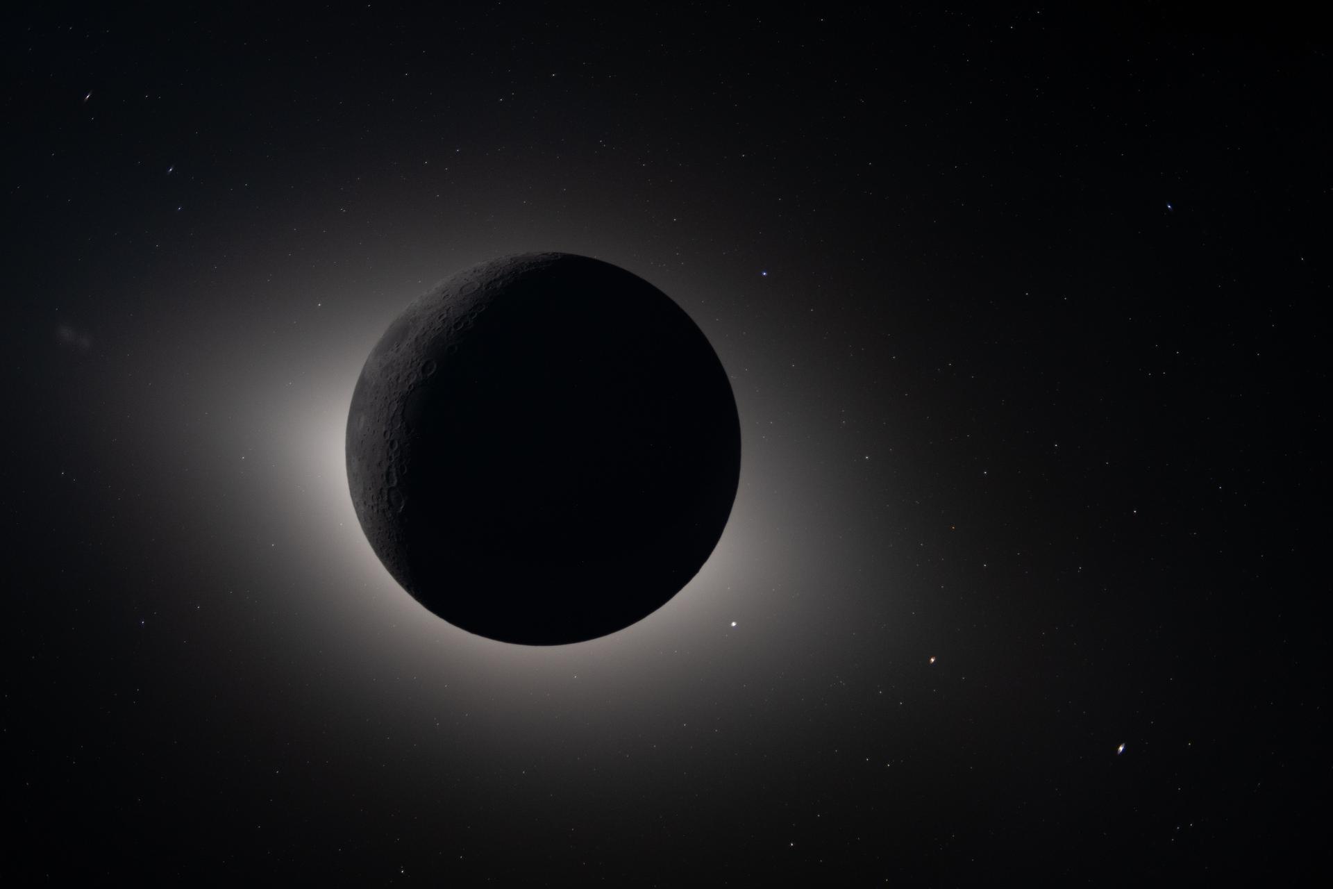
Fig. 0 — The original image. Art002e009301, 1920 × 1280 px. The Moon disc (black) is surrounded by what NASA describes as a glowing halo. Stars are clearly visible in the background, and a faint hint of earthshine is visible on the lunar limb.
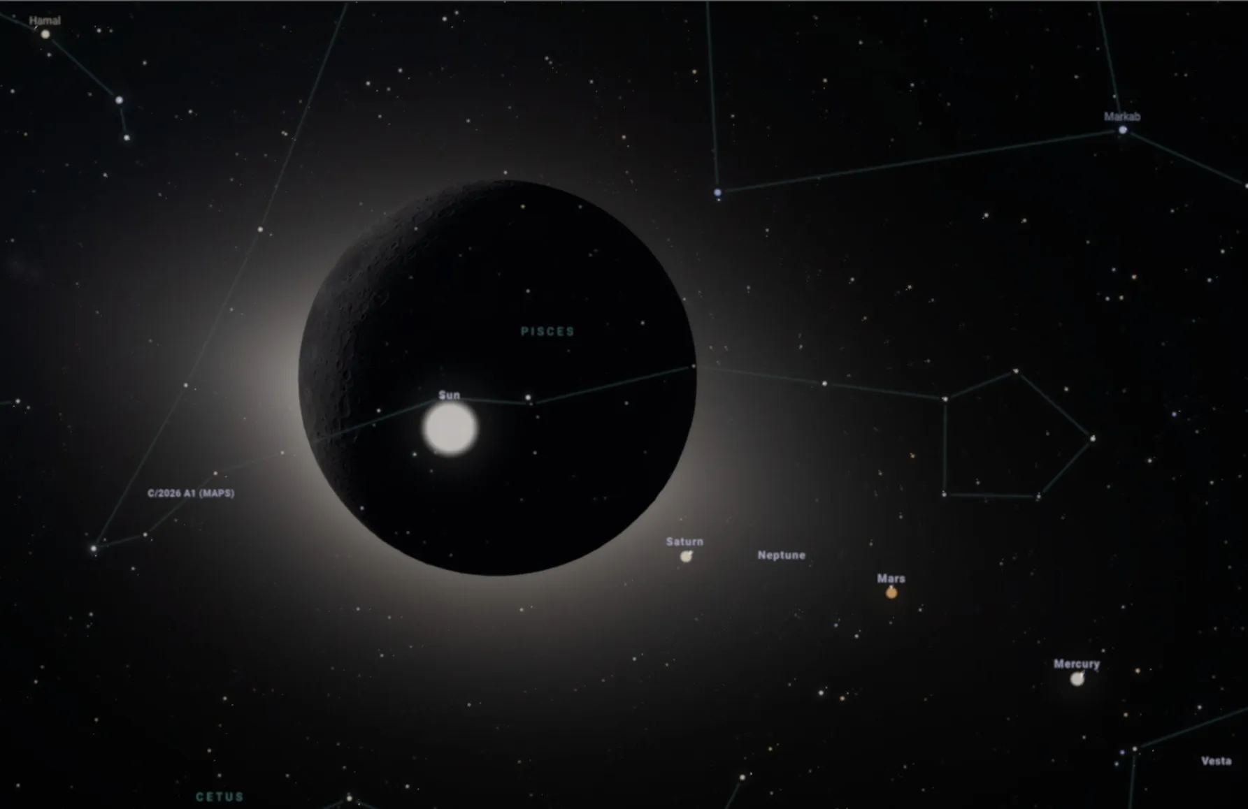
Fig. 0b — Eamonn Kerins' overlay of the eclipse image on a Stellarium field-of-view map (posted to Bluesky, 7 April 2026). This is the starting point for identifying the ecliptic orientation.
§2 Step 1 — Finding the Moon's disc centre
Before doing any photometric analysis I need a reliable (sub-pixel) estimate of the Moon's disc centre and radius. The obvious difficulty is that the dark disc and the dark background are both near-black, so simple thresholding won't separate them. The approach I settled on:
Radial ray-casting
- Start from a rough initial guess for the centre (x₀ = 754, y₀ = 653) from visual inspection.
- Cast 720 equally-spaced rays outward (0.5° angular resolution), sampling at every pixel from r = 150 px to r = 600 px.
- Along each ray, record the first pixel whose brightness exceeds a threshold of 35/255 — this is the dark-disc → bright-corona transition, i.e. the limb.
- Only keep limb points whose x-coordinate falls in the range 800 – 1100 px, i.e. the clean right-hand arc where the corona is well illuminated and unambiguous. This discards the left side where artefacts and the dark sky confused earlier approaches.
Pratt algebraic circle fit
A Pratt least-squares circle fit is applied to all accepted limb points. This is a numerically stable algebraic method that simultaneously solves for centre (cx, cy) and radius r. The system being solved is:
Iterative refinement
After the first fit I re-cast all rays from the new centre and refit. This is repeated until the change in centre or radius drops below 0.05 px — which typically happens after 3 iterations. The final result:
| Quantity | Value |
|---|---|
| Centre (image coords) | ≈ (784, 646) px |
| Disc radius | ≈ 283 px |
| Offset from image centre | x: −176 px, y: −14 px (Moon slightly left of frame centre) |
| Limb points used in fit | ~230 (right-arc only) |
The coordinate system for all subsequent analysis is centred on the fitted disc centre: x positive to the right, y positive upward (mathematical convention, not image convention).
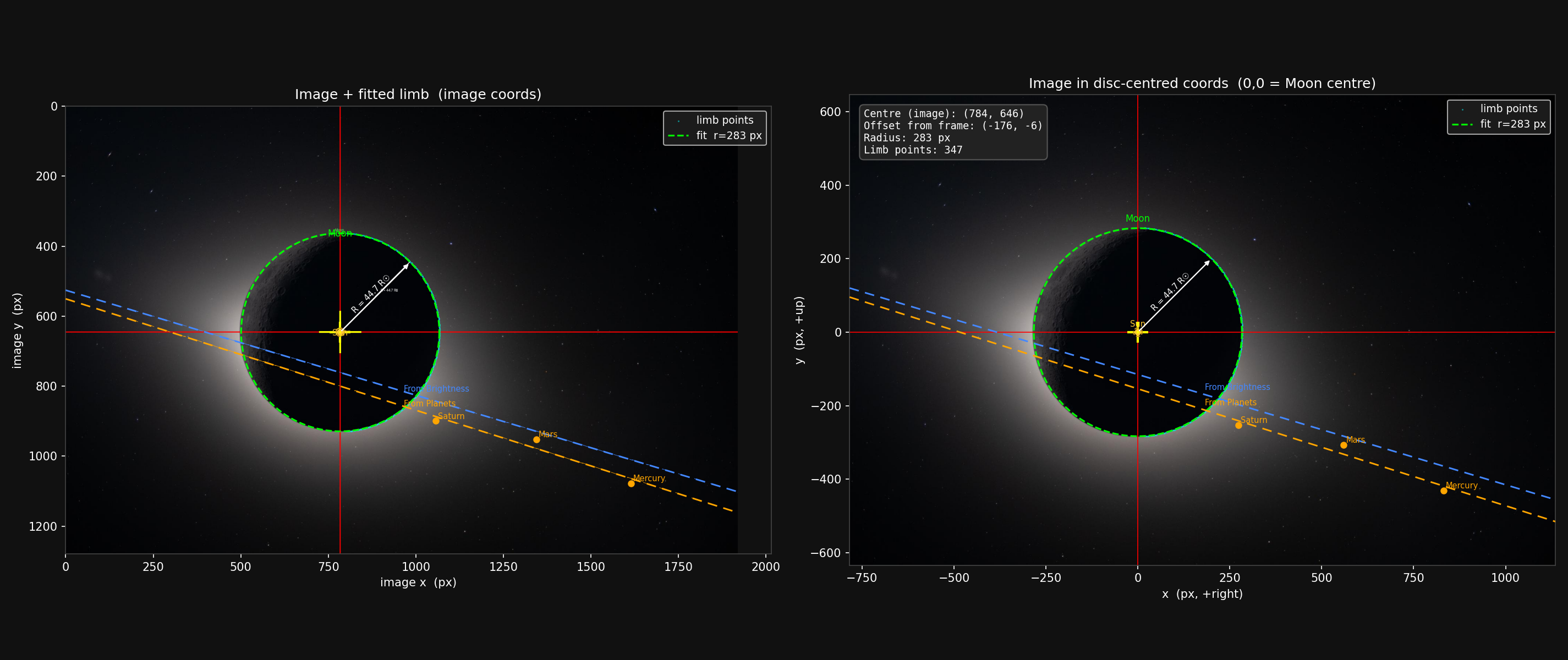
Fig. 1 — Disc centre determination (Method 1, moon-centred). Left: original image with cyan limb-point scatter and lime dashed fitted circle. Yellow crosshair marks the fitted centre. The blue dashed line is the manually adjusted "From Brightness" ecliptic estimate; the orange dashed line is the polyfit through Saturn, Mars and Mercury positions (see §5). Right: the same image plotted in disc-centred coordinates (0, 0 = Moon centre); red crosshairs confirm the alignment.
§3 Step 2 — How far out are we looking?
This is the key question for whether any coronal emission could plausibly be present. The Artemis II closest approach was 4,067 miles (6,545 km) above the lunar surface, so the Orion capsule was about 8,282 km from the Moon's centre.
Moon/Sun angular size ratio
From that distance, I can work out how large the Sun appears behind the Moon using the Moon's known physical radius as the angular ruler:
The result: the Moon's disc in this image is roughly 44.7 solar radii in angular size. The golden circle drawn in the figures shows the estimated position and apparent size of the Sun behind the Moon's centre, with dashed circles for upper and lower bounds based on uncertainty in when during the flyby the image was taken (ranging from 8,282 km at closest approach to ~15,000 km farther along the trajectory).
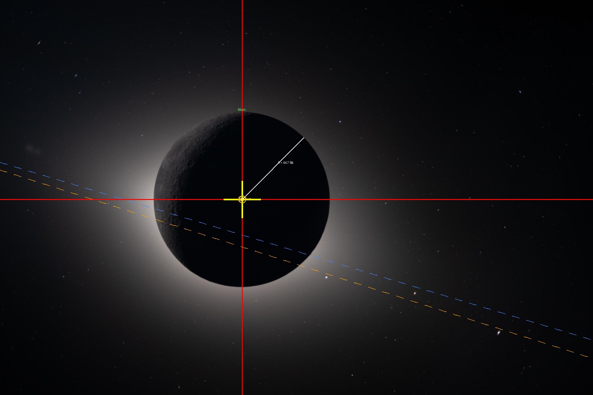
Fig. 2 — Annotated image (Method 1). Yellow crosshair at the Moon's fitted centre, which is also where the Sun is assumed to be. The solid gold circle shows the best-estimate apparent size of the Sun (r ≈ 6.3 px in this image), with dashed circles for the uncertainty range. The radial arrow is labelled R = 44.7 R☉. The two dashed lines mark the ecliptic estimates (blue = brightness-guided manual fit; orange = planet polyfit).
§4 Step 3 — Radial detrending
The raw image brightness falls off steeply with distance from the disc centre (mostly stray light / F-corona / zodiacal light). To reveal any faint structure I applied four standard radial filters. All filters work in the disc-centred coordinate system.
The four filters
① Power r³
Multiply each pixel by (r / Rdisc)3. The exponent compensates for the steep radial fall-off of coronal brightness. Higher powers bring up faint outer structure at the cost of saturating close-in features. I chose n = 3 as a starting point — it's a common value in eclipse work and seems to give a reasonable dynamic range here. Normalised to [0, 1] at the 0.5th and 99.5th percentiles to avoid hot pixels dominating the stretch.
② Newkirk (1961) model filter
Divides the image by a physical model of K-corona brightness (Newkirk 1961):
Dividing by the model "flattens" the expected radial gradient, making genuine deviations from the average K-corona profile stand out. It's not a perfect physical model at these large distances (~45 R☉) but still useful as a detrending baseline.
③ NRGF — Normalised Radial Gradient Filter
The NRGF (Morgan & Druckmüller 2006) takes a purely empirical approach: for each radial distance r, it subtracts the mean brightness of that annulus and divides by its standard deviation. Every radius is brought to zero mean / unit variance simultaneously:
The per-annulus statistics are computed in integer-pixel radius bins and lightly smoothed (uniform filter, width 5) to avoid noisy rings. This method is excellent for revealing tangential structure like streamers, because it is self-calibrating at every radius.
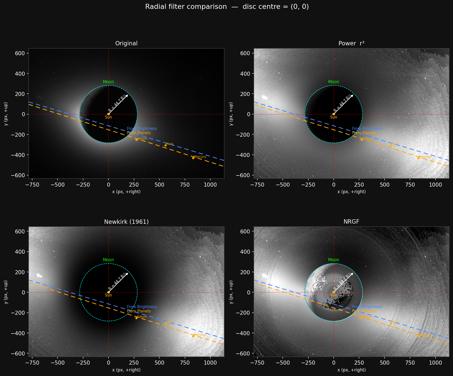
Fig. 3 — Radial filter gallery (Method 1, moon-centred). All four panels share the same disc-centred coordinate system (0, 0 = Moon centre, red crosshairs). The cyan dashed circle marks the fitted Moon limb; the gold circles show the estimated Sun size. The dashed lines are the ecliptic estimates (blue = brightness fit, orange = planet fit). Note the elongated band of brightness visible in the Power r³, Newkirk, and NRGF panels — this is the feature discussed in §5.
Of the four methods, the NRGF seems to best capture what looks like genuine structure: the band running along the ecliptic direction stands out most clearly once each radial annulus is independently normalised, because this removes the rotationally-symmetric component and leaves behind azimuthal variations. That is exactly what you would expect from a planar dust structure — the F-corona / Zodiacal Dust Cloud — whose symmetry plane is tilted a few degrees relative to the ecliptic and whose brightness is strongly concentrated toward the Sun–ecliptic direction.
§5 Step 4 — The plane of enhanced brightness
Looking at the Power r³, Newkirk, and NRGF panels, there is a fairly clear elongated band of enhanced brightness that runs diagonally across the image. It's not a perfectly clean feature — there's a lot of pixel-scale noise — but it's persistent across different filtering methods, which gives me some confidence it's real and not a filtering artefact.
Approach A — manual brightness fit ("From Brightness")
I drew a dashed line (blue in all figures) defined by a single point and slope in disc-centred coordinates, adjusted by eye until it passes through the visible band of enhanced brightness across multiple filter panels. This is entirely subjective — I'm just trying to capture the ridge of the feature by eye:
I iterated the slope and intercept a few times by editing the constants in the script and re-running. It's not a formal measurement — the feature is diffuse and the "best" line is somewhat a matter of judgement.
Approach B — planet positions fit ("From Planets")
If this feature is zodiacal light, it should lie along the ecliptic plane. To test this, I used the Stellarium overlay (from Eamonn Kerins' Bluesky post) to identify Saturn, Mars and Mercury in the image, and then clicked their positions directly on the eclipse JPEG using an interactive script. Their disc-centred positions came out as:
| Planet | Image coords (px) | Disc-centred (px) |
|---|---|---|
| Saturn | (1057, 899) | (+273, −253) |
| Mars | (1344, 952) | (+560, −306) |
| Mercury | (1615, 1078) | (+831, −432) |
A linear fit through these three points gives:
Reassuringly this is very close to the manually-estimated slope of −0.30 from the brightness feature alone, which is a decent sanity check that the feature really is aligned with the ecliptic. The orange dashed line in all figures shows this planet-based ecliptic estimate.
§6 Method 2 — Sun-centred analysis
I also tried an alternative coordinate system centred on the Sun's position rather than the Moon's centre. This is arguably more physically meaningful for a corona / zodiacal light analysis, since the radial filter should ideally be centred on the brightness source.
The Sun's position was identified in the Stellarium reference image
(via click_objects.py), then scaled from Stellarium image
coordinates to eclipse image coordinates. In disc-centred coordinates the
Sun sits at approximately (−90, −35) px — shifted slightly down-left from
the Moon centre, as expected from the geometry.
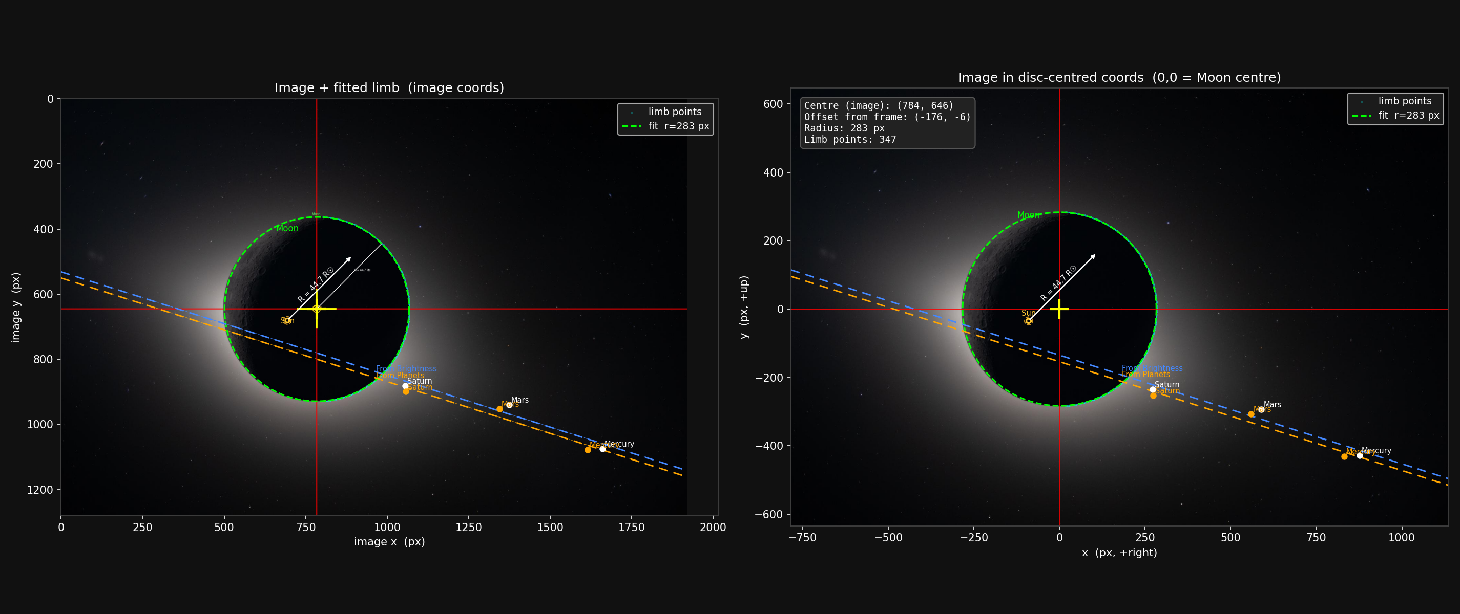
Fig. 4 — Method 2 (scaled coordinates), Figure 1.
Sun centre shifted by (~−90, −35) px in disc-centred coordinates. The
planet markers (white) come from objects.txt (Stellarium
image, scaled); orange markers from planets.txt (clicked
directly on eclipse image).
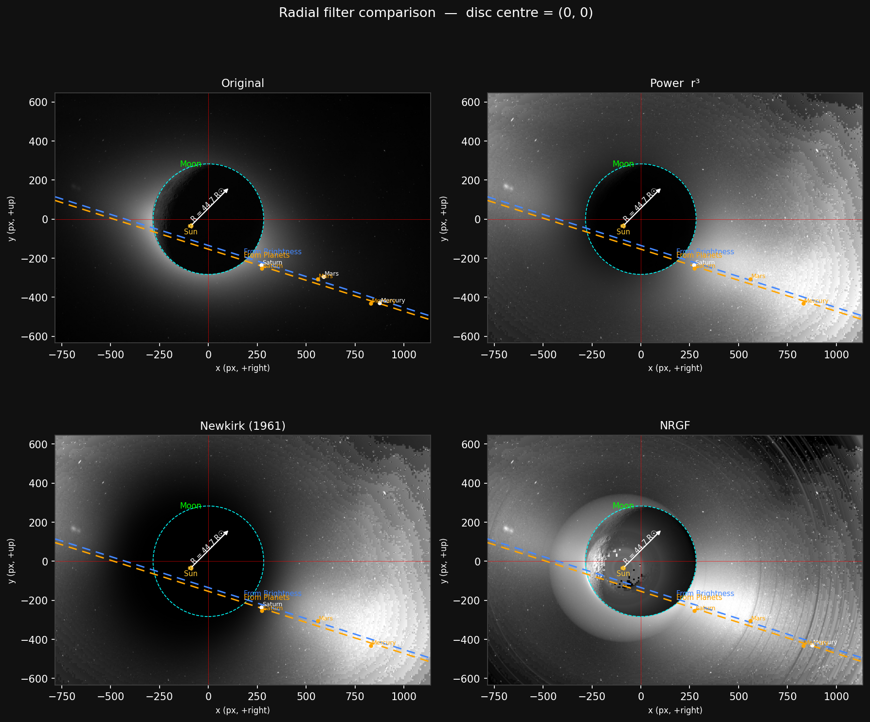
Fig. 5 — Method 2 radial filter gallery. The radial filters are now centred on the estimated Sun position rather than the Moon centre. Qualitatively the results look similar to Method 1, suggesting the brightness gradient is not particularly sensitive to the small offset between Moon and Sun centres — as you'd expect at ~45 R☉.
The results from Method 1 and Method 2 look quite similar: at 45 R☉ the ~90 px offset between Moon and Sun centres is less than 0.5% of the radial distance, so it barely changes the gradient correction. Method 1 is probably the more reliable choice here, because the stray-light contribution from the lunar occulter is centred on the Moon — not the Sun — making the radial brightness profile inherently asymmetric about the solar position. Detrending centred on the Moon therefore better captures and removes that component.
§7 Interpretation — dust scattering, not the K-corona
The NASA caption raised the question of whether the halo brightness is coronal. Here is the case for a dust-scattering origin, with the K-corona ruled out on geometric grounds alone.
1. The occulting scale rules out K-corona
At ~8,300 km from the Moon's centre, the Moon's disc subtends roughly 44.7 times the apparent solar radius. That means the nearest point of the corona visible in this image is about 44.7 R☉ from the solar centre. The K-corona (Thomson-scattered light from free electrons) falls off steeply with distance — roughly r−6 near the solar limb, transitioning to ~r−2.5 farther out (Baumbach 1937). It is essentially undetectable beyond ~5–10 R☉ even with dedicated coronagraphs. At 44 R☉ there is simply no K-corona signal to see.
2. The brightness profile matches the F-corona / zodiacal dust
Guillermo Stenborg (JHUAPL) noted that the brightness distribution looks very typical of white-light F-corona — sunlight Mie-scattered by interplanetary dust. The F-corona dominates over the K-corona beyond roughly 3–5 R☉ and merges smoothly into zodiacal light at larger elongations; at 45 R☉ the two labels describe the same physical phenomenon viewed at different angular distances from the Sun. There is likely also a contribution from stray light off the lunar occulter, particularly in the inner halo immediately surrounding the disc edge, though separating that component from genuine F-corona brightness would require a PSF model for the Orion camera system.
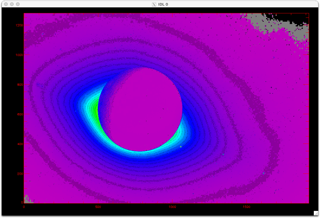
Fig. 6 — F-corona iso-contour analysis (G. Stenborg, JHUAPL). Rough brightness iso-contours overlaid on the eclipse image. The shape and radial gradient of the brightness distribution are strikingly similar to canonical white-light F-corona observations. In the absence of confounding factors (stray light, or the gravitational perturbation of Jupiter on the Zodiacal Dust Cloud), the centre of the iso-contour ellipses should coincide with the projected position of the Sun itself — offering an independent geometric check on the Sun's location in the image. The image also opens the door to measuring the inclination of the ZDC symmetry plane, the radial brightness gradient, and the eccentricity of the iso-contours as a function of radial distance.
3. Solar maximum argues against a coherent K-corona plane
Near solar maximum (April 2026), the corona is complex and roughly isotropic — multiple active regions and streamers distributed in all directions. A single coherent bright plane is inconsistent with a K-corona origin but perfectly consistent with the dust cloud, whose symmetry plane is fixed by orbital dynamics.
4. The plane geometry matches the ecliptic / ZDC symmetry plane
The direction of the brightness enhancement aligns closely (within ~1°) with the ecliptic plane as independently identified by fitting a line through Saturn, Mars and Mercury. The Zodiacal Dust Cloud is concentrated toward the ecliptic — with a small but measurable inclination relative to the invariable plane — and peaks strongly at low solar elongation. This makes it the natural explanation for a planar brightness feature at this geometry. The Stenborg iso-contours (Fig. 6) offer a route to measuring that inclination directly from this image.
§8 Unanswered questions & things I'd do next
- What is the true image orientation? EXIF / telemetry needed to confirm roll angle and tie the image frame to J2000.
- Where exactly was Orion when the image was taken? The image timestamp and trajectory data would pin down the exact Sun–Moon–camera geometry and improve the solar radius calculation.
- Can the iso-contour centre fix the Sun's position? Stenborg's analysis (Fig. 6) suggests yes — fitting elliptical iso-contours could give an independent measure of the Sun's projected position, cross-checked against the planet-based ecliptic line.
- What is the inclination of the ZDC symmetry plane? The orientation of the iso-contour major axis relative to the ecliptic encodes the tilt of the Zodiacal Dust Cloud — measurable if the image orientation is known.
- How does brightness fall off radially? A quantitative radial profile (with the stray-light component modelled out) could be compared to canonical F-corona photometry from LASCO or STEREO.
- How eccentric are the iso-contours as a function of radius? Eccentricity varying with elongation could reveal the dust cloud's geometric flattening and any asymmetry introduced by Jupiter's gravitational influence on the ZDC.
- Can the inner halo be separated from the F-corona? This requires a PSF model for the Orion camera to disentangle stray light from genuine dust-scattered brightness.
- Better planet coordinates. More precise astrometry (e.g. from a deeper Stellarium match or a plate-solve) would reduce slope uncertainty from ~1–2° down to a fraction of a degree.
Anyway — these are just quick notes. If any of this is interesting or obviously wrong, I'd genuinely welcome feedback.
App. Software & methods summary
All analysis was done in Python 3 with NumPy, Pillow, OpenCV,
Matplotlib and SciPy. The main script is
find_disc_centre.py; interactive planet-clicking tools
are click_objects.py (Stellarium image) and
click_planets.py (eclipse image). Run all combinations
with ./run_all.sh (non-interactive batch mode via
Matplotlib's Agg backend).
| Script | Purpose | Output |
|---|---|---|
find_disc_centre.py |
Disc fitting, radial filters, ecliptic lines, all figures | *_annotated.jpg, *_plot.png, *_filters.png |
click_objects.py |
Interactive: click Sun + planets on Stellarium image | objects.txt |
click_planets.py |
Interactive: click Saturn/Mars/Mercury on eclipse JPEG | planets.txt |
run_all.sh |
Batch: all combinations of Method × SCALE_PIXELS | 9 output files (3 runs × 3 images each) |
| Output suffix | Method | Description |
|---|---|---|
_m1 | 1 | Moon-centred (default, recommended) |
_m2_scaled | 2 | Sun-centred, Stellarium coords scaled to image size |
_m2_noscale | 2 | Sun-centred, Stellarium coords used as-is |