
|
|---|
Overview
 The Magnetohydrodynamic Algorithm outside a Sphere (MAS) code integrates the
time-dependent resistive thermodynamic magnetohydrodynamic (MHD) equations in
three-dimentional spherical coordinates and is used extensively in models of
coronal structure
[Mikić and Linker (1996),
Mikić et al. (1999),
Linker et al. (1999),
Lionello et al. (2008),
Downs et al. (2013) ,
Mikić et al. (2018)],
coronal dynamics
[Lionello et al. (2003),
Lionello et al. (2006),
Linker et al. (2011)],
and coronal mass ejections out to the Earth
[Linker et al. (2003),
Lionello et al. (2013),
Török et al. (2018)].
It is the primary MHD model in CORHEL (Corona-Heliosphere), a suite
of models for describing the solar corona and inner heliosphere [Riley et al. (2012)] and CORHEL-CME, an interface-based system for modeling CME eruptions from the Sun to Earth, both of which are available for public runs-on-demand at NASA's
Community Coordinated Modeling Center.
The Magnetohydrodynamic Algorithm outside a Sphere (MAS) code integrates the
time-dependent resistive thermodynamic magnetohydrodynamic (MHD) equations in
three-dimentional spherical coordinates and is used extensively in models of
coronal structure
[Mikić and Linker (1996),
Mikić et al. (1999),
Linker et al. (1999),
Lionello et al. (2008),
Downs et al. (2013) ,
Mikić et al. (2018)],
coronal dynamics
[Lionello et al. (2003),
Lionello et al. (2006),
Linker et al. (2011)],
and coronal mass ejections out to the Earth
[Linker et al. (2003),
Lionello et al. (2013),
Török et al. (2018)].
It is the primary MHD model in CORHEL (Corona-Heliosphere), a suite
of models for describing the solar corona and inner heliosphere [Riley et al. (2012)] and CORHEL-CME, an interface-based system for modeling CME eruptions from the Sun to Earth, both of which are available for public runs-on-demand at NASA's
Community Coordinated Modeling Center.
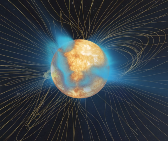
To develop a realistic model, photospheric magnetic field observations are used to specify the boundary condition on the radial magnetic field (Br). This data is taken from measurements at the Wilcox Solar Observatory, the Mount Wilson Observatory, the GONG and SOLIS instruments from the National Solar Observatory, the SOI/MDI instrument aboard the SOHO spacecraft, the HMI instrument aboard the SDO spacecraft, or the PHI instrument aboard the SolO spacecraft. The resulting solution provides a three-dimensional description of the coronal and/or heliospheric plasma and magnetic fields.
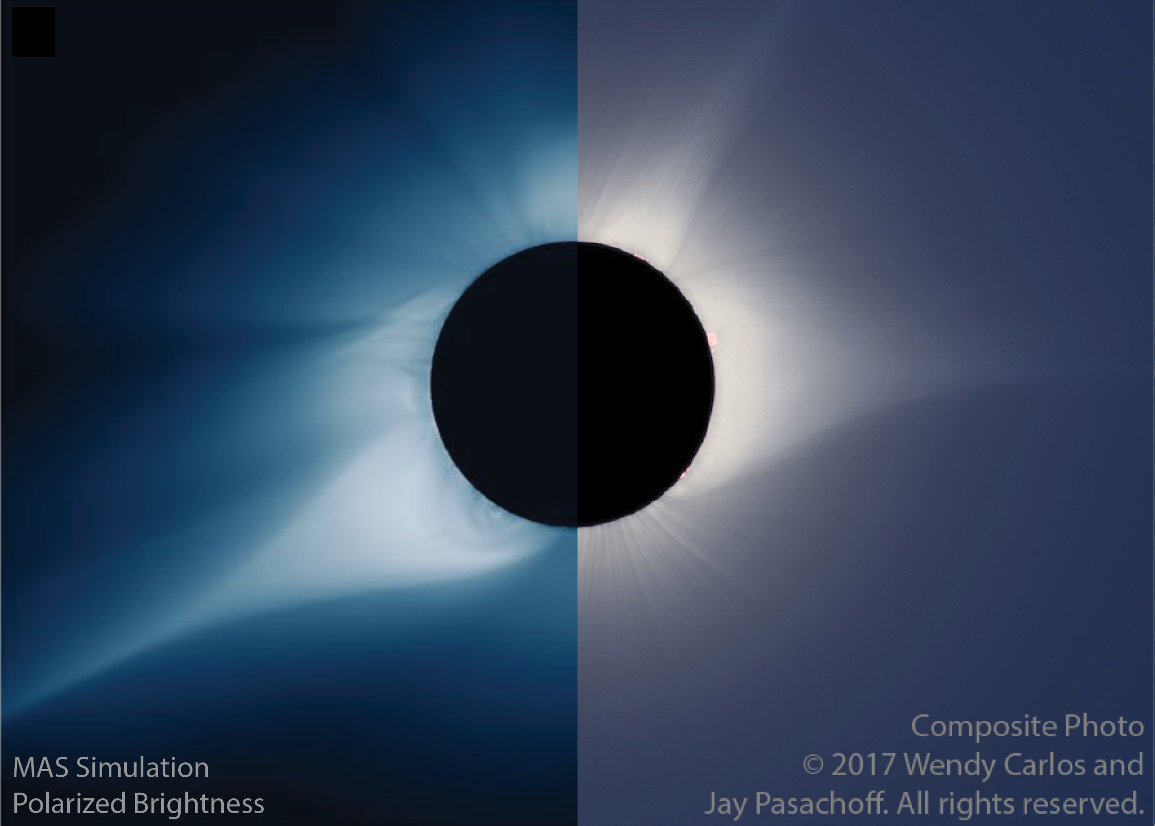 To compare the results with observations, we calculate synthetic observables
that can be quantitatively compared with ground and space-based observations.
For example, from the simulated electron density, we compute the total and polarized
brightness of the K-Corona in white light. The white light corona is best observed on the
ground during total solar eclipses, but it is also observed by coronographs, such as the
HAO Mauna Loa Coronameter,
and in space by the
LASCO coronagraph
aboard SOHO,
the
SECCHI
COR1,
and
COR2
coronagraphs and
HI
heliospheric imager aboard
STEREO,
and the
WISPR
instrument aboard
Parker Solar Probe.
Using the model density and temperature, we also synthesize EUV and soft X-ray
emission as observed in space, from instruments like
EIT
aboard
SOHO,
EUVI
aboard
STEREO,
XRT
aboard
Hinode,
and
AIA
aboard
SDO.
Direct comparisons of plasma and magnetic field properties can be made with
in-situ measurements from spacecraft such as
OMNI,
STEREO,
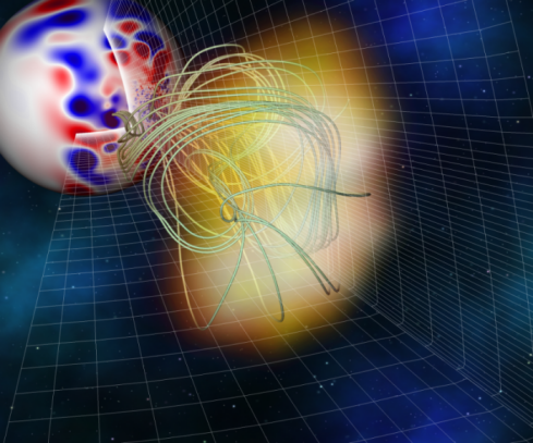
and Parker Solar Probe. We also visualize structural and topological features of
the magnetic field, such as open field regions
and the squashing factor "Q"
[Titov (2007)].
To compare the results with observations, we calculate synthetic observables
that can be quantitatively compared with ground and space-based observations.
For example, from the simulated electron density, we compute the total and polarized
brightness of the K-Corona in white light. The white light corona is best observed on the
ground during total solar eclipses, but it is also observed by coronographs, such as the
HAO Mauna Loa Coronameter,
and in space by the
LASCO coronagraph
aboard SOHO,
the
SECCHI
COR1,
and
COR2
coronagraphs and
HI
heliospheric imager aboard
STEREO,
and the
WISPR
instrument aboard
Parker Solar Probe.
Using the model density and temperature, we also synthesize EUV and soft X-ray
emission as observed in space, from instruments like
EIT
aboard
SOHO,
EUVI
aboard
STEREO,
XRT
aboard
Hinode,
and
AIA
aboard
SDO.
Direct comparisons of plasma and magnetic field properties can be made with
in-situ measurements from spacecraft such as
OMNI,
STEREO,
and Parker Solar Probe. We also visualize structural and topological features of
the magnetic field, such as open field regions
and the squashing factor "Q"
[Titov (2007)].
The MAS Model
The MHD equations used in MAS are
\[
\begin{alignat}{2}
\frac{\partial {\bf A}}{\partial t} &= {\bf v} \times {\bf B}
-{\frac{c^2}{4\,\pi}\,{\color{lightblue}{\eta}}\,\nabla \times \nabla \times {\bf A}}
\\
\frac{\partial \rho}{\partial t} &=-\nabla\cdot(\rho\,{\bf v})
\\
\frac{\partial T}{\partial t} &=-\nabla\cdot(T\,{\bf v})-
(\gamma - 2)\left(T\,\nabla\cdot{\bf v}\right)+\left.\frac{(\gamma-1)}{2\,k}\frac{m_p}{\rho}\right[\left.-
\nabla\cdot\left({\bf \color{lightblue}{\widetilde{\color{white}{q_1}}}} + {\bf q_2}\right)
-\frac{\rho^2}{m_p^2}\,{\bf \color{lightblue}{\widetilde{\color{white}{Q}}}} + {\bf H}\right] \notag
\\
\rho\,\frac{\partial{\bf v}}{\partial t}& = -\rho\,{\bf v}\cdot \nabla\,{\bf v}
+ \frac{1}{c}\,{\bf J} \times {\bf B} - \nabla (p+p_w) + \rho\,{\bf g}
+ {\bf F_{c}}
+ \nabla\cdot({\color{lightblue}{\nu}}\,\rho\,\nabla {\bf v})
{\color{lightblue}{+ \nabla\cdot\left({\bf S}\,\rho\,\nabla{\frac{\partial \bf v}{\partial t}}\right)}} \notag
\end{alignat}
\]
where ${\bf A}$ is the magnetic vector potential,
$\rho$ is the plasma density,
$T$ is the temperature,
${\bf v}$ is the plasma velocity,
${\bf B}=\nabla\times {\bf A}$ is the magnetic field which satisfies the $\nabla \cdot {\bf B}=0$ condition,
${\bf J}=(c/4\pi)\,\nabla\times {\bf B}$ is the current density,
$p=2\,k\,T\,\rho/m_p$ is the plasma pressure,
$p_w$ is the Alfvén wave pressure (see below),
${\bf \color{lightblue}{\widetilde{\color{white}{q_1}}}}$ is the modified heat flux due to parallel Spitzer collisional thermal conduction (see below),
${\bf q_2}$ is the heat flux due to collisionless thermal conduction (see below),
${\bf \color{lightblue}{\widetilde{\color{white}{Q}}}}$ is the modified optically thin radiative loss function (see below),
${\bf H}$ is the coronal heating (see below),
$\gamma$ is the adiabatic index,
${\bf g}=-g_0\,R_{\odot}^2\,{\bf \hat r}/r^2$ is the gravitational force,
${\bf F_c}=\rho\,\left(2\,\Omega \times {\bf v} + \Omega \times \left(\Omega \times {\bf r}\right)\right)$ combines the Coriolis and centrifugal terms used when computing in the co-rotating frame,
$c$ is the speed of light in a vacuum,
$m_p$ is the proton mass,
$k$ is Boltzman's constant,
$\eta$ is the resistivity coefficient,
$\nu$ is the kinematic viscosity coefficient, and
${\bf S}$ is a semi-implicit factor (see below).
Terms colored light blue are added/modified for numerical efficiency and/or stability (see below).
The modified parallel Spitzer collisonal heat flux ${\bf \color{lightblue}{\widetilde{\color{white}{q_1}}}}$ [Spitzer and Harm (1953)] and collisionless heat flux ${\bf q_2}$ [Hollweg (1976)] are defined as \[ {\bf \color{lightblue}{\widetilde{\color{white}{q_1}}}} =f_{\mbox{c}}(r)\,\color{lightblue}{f_{\mbox{$\kappa$-mod}}(T)}\,\kappa_0\,T^{5/2}\, {\bf \hat b}{\bf \hat b}\cdot\nabla T, \qquad {\bf q_2}=(1-f_{\mbox{c}}(r))\,\frac{\alpha_{\mbox{nc}}\,k\,\rho}{(\gamma-1)\,m_p}\,T\,({\bf v}-\Omega\times {\bf r})\,{\bf \hat b}{\bf \hat b} \] where ${\bf \hat b}=|{\bf B}|/{\bf B}$ is the normalized direction of the magnetic field, $\kappa_0=9\times10^{-7}$ is the Spitzer parallel electron thermal conductivity constant, $\alpha_{\mbox{nc}}\sim O(1)$ is based on the deviation from Maxwellian of the solar wind's electron distribution, $f_{\mbox{c}}(r)=1/2-1/2\,\mbox{tanh}\left((r-r_{\mbox{tc}})/\sigma_{\mbox{tc}}\right)$ is a radial profile used to transition between collisional and collisionless thermal conduction, and $\color{lightblue}{f_{\mbox{$\kappa$-mod}}(T)}$ is a modification function used for resolving the transition region (see below).
Radiative LossesThe radiative loss function in MAS is \[ {\bf \color{lightblue}{\widetilde{\color{white}{Q}}}}={\bf Q}/\color{lightblue}{f_{\mbox{$\kappa$-mod}}(T)}, \] where ${\bf Q}$ is a selected temperature-dependent radiative loss function and $\color{lightblue}{f_{\mbox{$\kappa$-mod}}(T)}$ is a modification function used for resolving the transition region (see below). MAS contains multiple options for specifying the radiative loss function including [Rosner et al. (1978), Mok et al. (2004), Athay (1986)], as well as some directly based on the CHIANTI database. The CHIANTI options currently use version 7.1 [Landi et al. (2013)] through lookup tables based on coronal, photospheric, or hybrid abundances.
Heating
MAS contains numerous coronal heating models, both empirical and physics-based, that can be combined together.
Empirical heating can be set by a combination of analytic
functions
[e.g. Lionello et al. (2009)],
while the primary physics-based approach is the wave-turbulence-driven (WTD) model
[Lionello et al. (2014),
Downs et al. (2016),
Mikić et al. (2018)].
In the WTD approach, auxiliary equations are solved to describe the
large-scale evolution of turbulent Alfvénic fluctuations in the
corona and solar wind. This takes the form of two coupled PDEs
governing the evolution of the envelope of the fluctuation amplitudes ($z_{\pm}$)
via propagation, reflection, and dissipation:
\[
\frac{\partial z_{\pm}}{\partial t}
=-\left({\bf v}\pm {v_A}\right)\cdot\nabla\,z_{\pm}
+ \frac{z_{\pm}}{4}\left({\bf v} \mp {v_A}\right)\cdot\nabla\left(\mbox{ln}\,\rho\right)
+ \frac{z_{\mp}}{2}\left({\bf v} \mp {v_A}\right)\cdot\nabla\left(\mbox{ln}\left|{v_A}\right|\right)
- \frac{z_{\pm}\left|z_{\mp}\right|}{2\,\lambda_{\perp}},
\]
where the Alfvén wave speed is defined as $v_A^2=|{\bf B}|^2/(4\,\pi\,\rho)$ and
the Poynting flux of waves entering the domain is chosen
by setting a uniform outward wave amplitude $z_0$ at the lower boundary
($\left|z_{\pm}(r=R_{\odot})\right|=z_0$).
The WTD heating term takes the form of:
\[
H_{\mbox{wtd}}=\frac{\rho}{4\,\lambda_{\perp}}\,\left(|z_{-}|\,z_{+}^2 + |z_{+}|\,z_{-}^2\right)
\]
where $\lambda_{\perp}=\lambda_0\,\sqrt{{B_w}/{|{\bf B}|}}$ is the correlation length,
and $B_w=6.09\,\mbox{G}$ is a chosen reference magnetic field and $\lambda_0$ is a tunable parameter.
MAS can also solve for the Alfvén wave pressure using a more simplified approach than WTD. In this case, it is found by averaging the forward and backward Alfvén wave pressures as $p_w=\left(\epsilon_{+}+\epsilon_{-}\right)/2$ where $\epsilon{\pm}$ are computed by integrating the Wentzel-Kramers-Brillouin (WKB) approximation [Mikić et al. (1999)] for the wave energies: \[ \frac{\partial \epsilon_{\pm}}{\partial t} =-\nabla\cdot \left( \epsilon_{\pm}\left[{\bf v}\pm v_A\,{\bf \hat b}\right]\right) - \frac{1}{2}\,\epsilon_{\pm}\,\nabla\cdot {\bf v} \]
Modifications to the Model for Numerical Efficiency and/or Stability
The MAS code uses an adaptive time-step that conforms to the
plasma flow CFL condition. As this is often a much slower time-scale
than the magnetosonic wave travel time, a “semi-implicit ” term is added
to the velocity advance to provide unconditional linear stability for
time steps larger than the fast magnetosonic wave limit.
The term “semi-implicit ” is used in this context to refer to a term that
modifies the dispersion relations for MHD waves in a manner similar to a
fully implicit algorithm
[Schnack et al. 1987] and has also been
described as the approximate implicit approach
[Carmana et. al. (1991)].
The semi-implicit term is computationally advantageous compared to a
fully-implicit approach because it results in a symmetric positive
definite operator (easier to solve) and can be solved separately
(operator split) from other terms in the MHD equations.
The semi-implicit term is computed locally on the grid based on the
Alfvén and sound speeds, and in MAS is set as
[Lionello et al. (1999)]:
\[
\color{lightblue}{{\bf S(r,\theta,\phi)}=\frac{1}{\Delta t^2\,\tilde k^2}\,\left(\frac{C_w^2}{(1-C_f)^2} - 1\right)}
\]
where $\Delta t$ is the time-step,
$\tilde k = 2\,\left(\Delta r^{-2} + (r\,\Delta\theta)^{-2}+(r\,\Delta \phi\,\sin\theta)^{-2}\right)^{1/2}$,
$C_f=\Delta t\,\tilde k \cdot {\bf v}$ is the flow CFL,
and $C_w=(1/2)\,\Delta t\,\tilde k\,(v_c^2+v_A^2)^{1/2}$ is the wave CFL, where $v_c=(\gamma\,p/\rho)^{1/2}$
is the sound speed.
The semi-implicit term goes to zero in regions that are explicitly
stable for the selected time step, as well as in the limit of a
steady-state solution ($d/dt\rightarrow 0$).
Although stable, the wave-like terms do not guarantee monotonicity, resulting in the potential emergence of oscillatory behavior on the order of the grid size. In order to avoid such behavior (and to prevent physical structures smaller than the grid from trying to form), the dissipative resistivity $\color{lightblue}{\eta}$ and kinematic viscosity $\color{lightblue}{\nu}$ coefficients are set artificially higher than their physical values. However, to maintain accuracy, they are chosen such that the resulting diffusion time scales remain much larger than the typical Alfvén travel time. For flexibility, these coefficients can be constant or spatially-dependent.
Lastly, resolving the transition region between the lower chromosphere and the corona poses a difficult challenge for numerical models. Here, the temperature and density change by orders of magnitude over very little distance. Even with a non-uniform grid, resolving this region requires an exorbitant number of grid points. To alleviate this problem, we apply a smooth modification function to the Spitzer thermal conduction coefficient and its inverse to the radiative loss function [Lionello et al. (2009), Mikić et al. (2013)]: \[ {\bf \color{lightblue}{\widetilde{\color{white}{q_1}}}} = \color{lightblue}{f_{\mbox{$\kappa$-mod}}(T)}\,{\bf q_1}, \] \[ {\bf \color{lightblue}{\widetilde{\color{white}{Q}}}} = {\bf Q}/\color{lightblue}{f_{\mbox{$\kappa$-mod}}(T)}, \] where \[ \color{lightblue}{f_{\mbox{$\kappa$-mod}}(T) = \left(1+(T/T_{\mbox{cut}})^{-10}\right)^{1/4}} \] such that $\color{lightblue}{f_{\mbox{$\kappa$-mod}}(T)}\rightarrow 1$ for $T \gt T_{\mbox{cut}}$ and $\color{lightblue}{f_{\mbox{$\kappa$-mod}}(T)}\rightarrow (T/T_{\mbox{cut}})^{-5/2}$ for $T \lt T_{\mbox{cut}}$ (acting as a temperature cut-off function for ${\bf q_1}$ at temperatures below $T_{\mbox{cut}}$). This causes the transition region to broaden substantially while preserving the coronal solution above.
Numerical Methods
 The MAS code is written in Fortran
and parallelized for CPUs and GPUs
using Message Passing Interface (MPI)
, OpenACC, and Fortran's `do concurrent' standard parallelism [Caplan et al. (2023)].
It solves the MHD equations on a non-uniform
logically-rectangular staggered grid
using finite differences. The non-uniformity of the grid helps MAS to efficiently
resolve small-scale structures
such as the transition region and active regions, while allowing for coarser grid
points over the global scale. Each component of the field vectors are staggered which,
combined with the use of the vector potential as a primitive, guarantees that the
magnetic field is divergence-free. Advective terms are spatially differenced using
first-order upwinding, while parabolic and gradient terms are centrally differenced using `Method A' from
[Veldman and Rinzema (1992)].
The MAS code is written in Fortran
and parallelized for CPUs and GPUs
using Message Passing Interface (MPI)
, OpenACC, and Fortran's `do concurrent' standard parallelism [Caplan et al. (2023)].
It solves the MHD equations on a non-uniform
logically-rectangular staggered grid
using finite differences. The non-uniformity of the grid helps MAS to efficiently
resolve small-scale structures
such as the transition region and active regions, while allowing for coarser grid
points over the global scale. Each component of the field vectors are staggered which,
combined with the use of the vector potential as a primitive, guarantees that the
magnetic field is divergence-free. Advective terms are spatially differenced using
first-order upwinding, while parabolic and gradient terms are centrally differenced using `Method A' from
[Veldman and Rinzema (1992)].
Several time integration schemes are used in the model. Advective terms are integrated with an explicit predictor-corrector upwinding scheme [Lionello et al. (1999)] where any “reaction ” terms (such as heating, radiative loss, gravitational forces etc.) are computed in the corrector step. The semi-implicit term is solved in the predictor-corrector framework implicitly using two preconditioned conjugate gradient (PCG) solves, while diffusive-like terms (such as thermal conduction and viscosity) are operator-split and either solved implicitly with backward-Euler+PCG or explicitly with a second-order Runge-Kutta Gegenbauer (RKG2) super time-stepping scheme combined with a PTL time step limiting method [Caplan et al. (2024)]. The WKB Alfvén wave pressure advance is operator split and integrated with the forward-Euler scheme sub-cycled at the Alfvén wave CFL limit. The wave turbulence advance is also operator split from the main MHD equations and sub-cycled, but uses a 2nd-order TVD Runge-Kutta time-stepping scheme [Gottlieb and Shu (1998)]. Within each step, we use Strang splitting of the various operators. A OSPRE flux-limiting scheme [Waterson and Deconinck (2007)] is used for the advective operators, while a point-implicit scheme is used for the remaining operators [Tóth et al. (2012)].
The PCG solver in MAS has two communication-free preconditioning options. Depending on the problem, we either use a non-overlapping domain decomposition with zero-fill incomplete LU factorization [Saad (2003)] or point-Jacobi (diagonal scaling). The operator matrices are stored in a modified diagonal (DIA) sparse storage format for internal grid points, while the boundary conditions are applied matrix-free. The preconditioner matrix is stored in a compressed sparse row (CSR) storage format optimized for vectorized memory access [Smith and Zhang].
The code exhibits parallel strong scaling up to thousands of CPU cores (MPI ranks) on large HPC systems. A 3D decomposition is used to distribute to domain across MPI ranks in a topologically-aware communicator. Inter-rank communication is performed asynchronously whenever possible. A hybrid MPI+STDPAR+OpenACC approach is used to scale the code to multiple GPU compute nodes [Caplan et al. (2023)].
 Return to PSI's Coronal Modeling Page