Interpolating Datasets

Interpolate slices from standard PSI data files.

This example demonstrates how to use

• np_interpolate_slice_from_hdf(),

• interpolate_positions_from_hdf(),

from pathlib import Path
from psi_io import data, read_hdf_meta, np_interpolate_slice_from_hdf, interpolate_positions_from_hdf
import matplotlib.pyplot as plt
import numpy as np

Read in the metadata for a 3D data file (the radial magnetic field data).

br_data_filepath = data.get_3d_data()
metadata = read_hdf_meta(br_data_filepath)

Datasets for file: br.h5
+-----------------+-----------------+-----------------+
| Name            | Shape           | Type            |
+-----------------+-----------------+-----------------+
| Data            | (181, 100, 151) | float32         |
+-----------------+-----------------+-----------------+

Scales for file: br.h5
+------------+------------+------------+------------+------------+------------+------------+
| Dataset    | Dim        | Name       | Shape      | Type       | Min        | Max        |
+------------+------------+------------+------------+------------+------------+------------+
| Data       | 0          | dim1       | (151,)     | float32    | 0.99956024 | 30.511646  |
| Data       | 1          | dim2       | (100,)     | float32    | 0.0        | 3.1415927  |
| Data       | 2          | dim3       | (181,)     | float32    | 0.0        | 6.2831855  |
+------------+------------+------------+------------+------------+------------+------------+

Using this metadata, we can see that the dataset is a standard PSI 3D data file with scales:

• radius (1st dimension), in units of solar radii (R☉),

• co-latitude (2nd dimension), in radians,

• longitude (3rd dimension), in radians.

Suppose we wish to interpolate the given dataset at a specific radial value, say at 30 R☉, across all latitudes and longitudes. The most efficient approach is through the function np_interpolate_slice_from_hdf(), which uses vectorized NumPy computation for interpolation, while also leveraging read_hdf_by_value() to only read in the minimum amount of data to perform these computations.

data_at_30 = np_interpolate_slice_from_hdf(br_data_filepath, 30, None, None)
for r in data_at_30:
    print(r.shape)

(181, 100)
(100,)
(181,)

Note

np_interpolate_slice_from_hdf() results in a dimensional reduction of the dataset. In this case, the original 3D dataset is reduced to a 2D slice at the specified radial value.

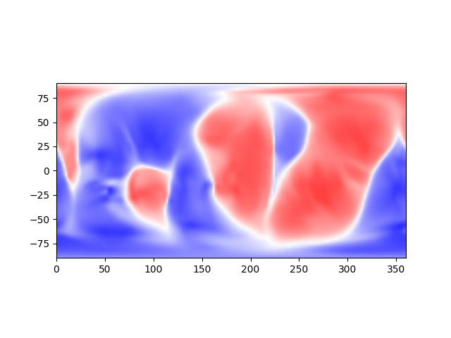
Given the metadata fetched above, we can visualize this slice as a long-lat map:

data, scale_t, scale_p = data_at_30

ax = plt.figure().add_subplot()
ax.pcolormesh(np.rad2deg(scale_p),
              90-np.rad2deg(scale_t),
              data.T,
              cmap='bwr',
              shading='gouraud',
              clim=(-5e-4,5e-4))
ax.set_aspect("equal", adjustable="box")
plt.show()

Alternatively, if we wish to interpolate the dataset at arbitrary (radius, co-latitude, longitude) positions, we can use interpolate_positions_from_hdf(). For example, to interpolate at some (contrived) trajectory:

r_positions = np.linspace(1.0, 30.0, 10)  # from 1 R☉ to 30 R☉
theta_positions = np.linspace(0.0, np.pi, 10)  # from
phi_positions = np.linspace(0.0, 2*np.pi, 10)  # from 0 to 2π
interpolated_values = interpolate_positions_from_hdf(
    br_data_filepath,
    r_positions,
    theta_positions,
    phi_positions
)

for value, position in zip(interpolated_values, zip(r_positions, theta_positions, phi_positions)):
    print(f"(radius={position[0]:.2f} R☉, "
          f"latitude={90-np.rad2deg(position[1]):.2f}°, "
          f"longitude={np.rad2deg(position[2]):.2f}°) ->\n"
          f"    B_r = {value:.4e} MAS UNITS")

(radius=1.00 R☉, latitude=90.00°, longitude=0.00°) ->
    B_r = 3.3264e-01 MAS UNITS
(radius=4.22 R☉, latitude=70.00°, longitude=40.00°) ->
    B_r = -2.4614e-03 MAS UNITS
(radius=7.44 R☉, latitude=50.00°, longitude=80.00°) ->
    B_r = -4.8336e-03 MAS UNITS
(radius=10.67 R☉, latitude=30.00°, longitude=120.00°) ->
    B_r = -2.4804e-03 MAS UNITS
(radius=13.89 R☉, latitude=10.00°, longitude=160.00°) ->
    B_r = 7.3004e-04 MAS UNITS
(radius=17.11 R☉, latitude=-10.00°, longitude=200.00°) ->
    B_r = 1.0084e-03 MAS UNITS
(radius=20.33 R☉, latitude=-30.00°, longitude=240.00°) ->
    B_r = 6.2016e-04 MAS UNITS
(radius=23.56 R☉, latitude=-50.00°, longitude=280.00°) ->
    B_r = 3.9668e-04 MAS UNITS
(radius=26.78 R☉, latitude=-70.00°, longitude=320.00°) ->
    B_r = -2.3550e-04 MAS UNITS
(radius=30.00 R☉, latitude=-90.00°, longitude=360.00°) ->
    B_r = -1.9969e-04 MAS UNITS