EUV image preprocessing data
Here we provide limb-brightening correction (LBC) and inter-instrument transformation (IIT) parameters for STEREO-A/B EUVI 195Å and SDO AIA 193Å. The data is provided for use with both the original level-1 data from SSW, and for the same data after being PSF deconvolved.
If you wish to use the preprocessing data with PSF deconvolved images, the PSFs you use for STEREO-A/B EUVI should be obtained from SSW, while those for AIA should be obtained from [B. Poduval et al.]. In order to match the preprocessing data to the PSF-deconvolved images precisely, the deconvolutions should be performed using the SGP algorithm implemented by [Prato, M. et al.] for 11 iterations. See [here] for the author's freely available SGP-IDL code.
For all data sets, an EUV disk image radius of \(R_0=1.01\;R_{\odot}\) is assumed.
The data is provided in MATLAB's native mat format and hdf4 format. The IIT data is also provided in ascii text format.
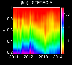
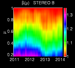
Limb-brightening correction (LBC)
Limb brightening corrections aim to make every region of an EUV emission image to appear as if it were viewed at disk center, eliminating the increase in image intensity of structures towards the disk edges.
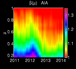
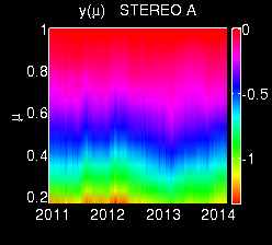
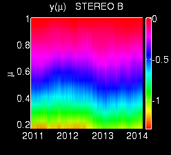
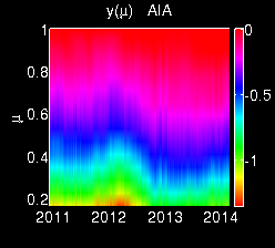
Given an EUV image \(F\), we define \(I=\mbox{log}_{10}F\), and the limb-brightening correction transformation is applied as
\[ I^{\prime}(\mu) = \beta(\mu)\,I(\mu) + y(\mu), \]
where \(I^{\prime}\) is the corrected image, and \(\mu = \cos \theta\) and \(\theta\in[0, \pi/2]\) is the angle from disk center to the limb. The computed values for \(\beta(\mu)\) and \(y(\mu)\) from 12/10/2010 to 02/17/2014 at 6-hour cadence are provided below. They are provided for both SSW level-1 images and PSF deconvolved images (see above for details).
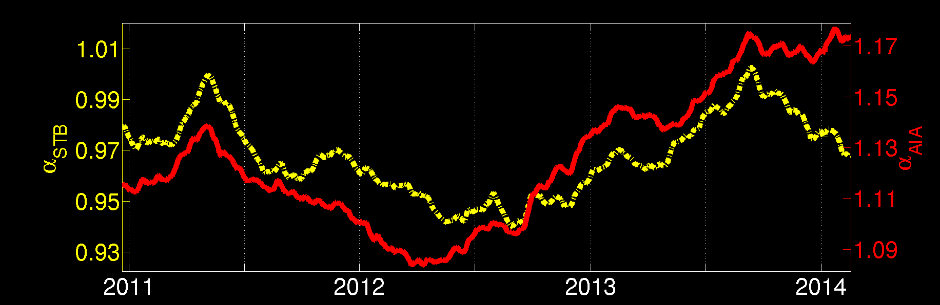
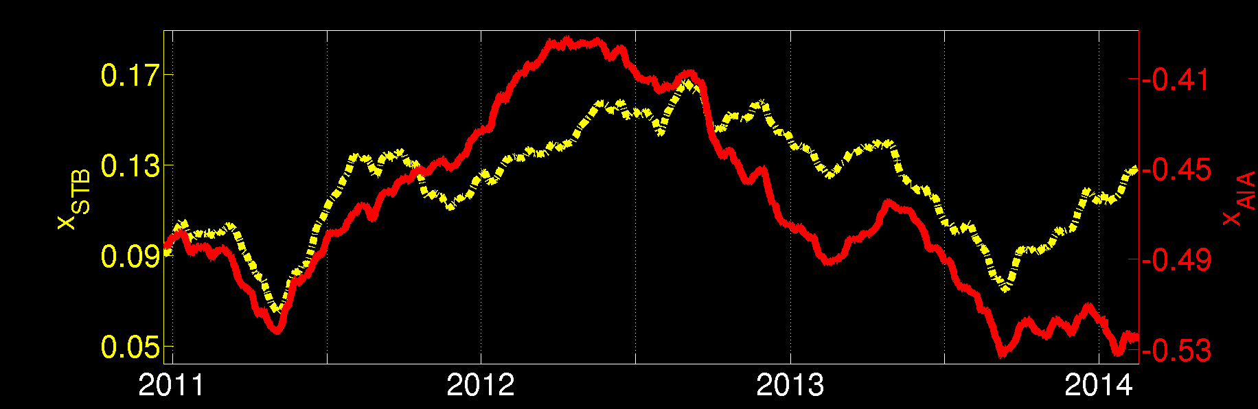
Inter-instrument transformations (IIT)
The inter-instrument transformations (IIT) aim to transform EUV disk images from STEREO-B EUVI 195Å and AIA 193Å to appear as if they were imaged using STEREO-A EUVI 195Å. This way, the three instruments' images can be combined to create synchronic EUV maps, and can be processed by coronal hole detection software using the same thresholding parameters.
We apply the IIT transformation as
\[ I^{\prime} = \alpha\,I + x, \]
where \(I\) is a \(\mbox{log}_{10}\) image from an instrument other than STEREO-A EUVI 195Å and \(I^{\prime}\) is the transformed \(\mbox{log}_{10}\) image which appears as if it was produced by STEREO-A EUVI 195Å. The computed values for \(\alpha\) and \(x\) from 12/21/2010 to 02/17/2014 at 6-hour cadence are provided below.
There are four data sets available, depending on whether or not the images being transformed have been PSF deconvolved, and whether or not they have been limb-brightening corrected using the above LBC data (see above). The recommended approach is to use data which has been both PSF deconvolved and LBCC corrected. However, if you wish to apply the IIT to original level-1 SSW data, simply choose option (d) in the pull-down menu.