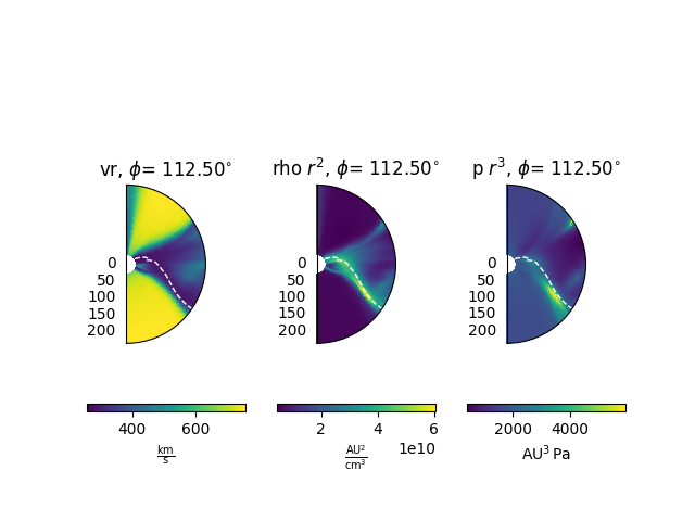
Plotting constant longitude slices

This example shows how to plot slices of constant longitude from a MAS model output.

First, load the required modules.

from psipy.model import MASOutput
import matplotlib.pyplot as plt

Next, load a set of MAS output files. You will need to change this line to point to a folder with MAS files in them.

mas_path = '/Users/dstansby/github/psipy/data/helio'
model = MASOutput(mas_path)

Each MAS model contains a number of variables. The variable names can be accessed using the .variables attribute.

print(model.variables)

Out:

['p', 't', 'va', 'br', 'vp', 'jp', 'jr', 'bp', 'vr', 'bt', 'vt', 'rho', 'jt']

Set parameters for plotting. The first line will give us a horizontal errorbar underneath the plots. The second line is the index to select for the longitude slice.

cbar_kwargs = {'orientation': 'horizontal'}
phi_idx = 40

Plot the slices

Note that for density (rho) and pressure (p) we first normalise the data relative to a power law decrease, to make it easer to see spatial variations.

fig = plt.figure()
axs = [plt.subplot(1, 3, i + 1, projection='polar') for i in range(3)]

ax = axs[0]
model['vr'].plot_phi_cut(phi_idx, ax=ax, cbar_kwargs=cbar_kwargs)

ax = axs[1]
rho = model['rho']
rho_r2 = rho.radial_normalized(2)
rho_r2.plot_phi_cut(phi_idx, ax=ax, cbar_kwargs=cbar_kwargs)

ax = axs[2]
p = model['p']
p_r3 = p.radial_normalized(3)
p_r3.plot_phi_cut(phi_idx, ax=ax, cbar_kwargs=cbar_kwargs)


# Add a contour of br = 0 (the heliopsheric current sheet) to all the axes
for ax in axs:
    model['br'].contour_phi_cut(phi_idx, levels=[0], ax=ax,
                                colors='white', linestyles='--', linewidths=1)

plt.show()