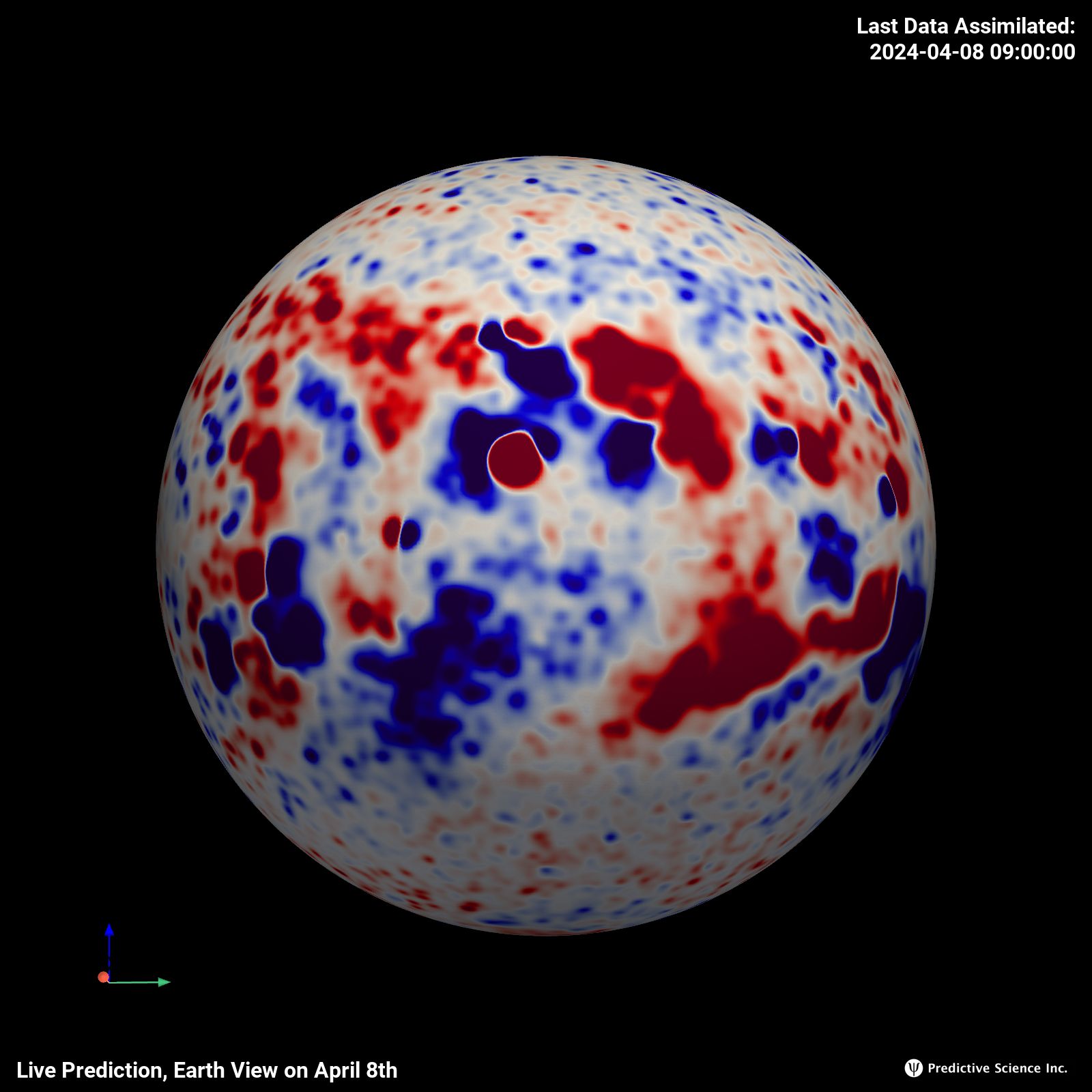
Br on the Sphere
(Surface Boundary Condition)

Volume Rendered Squashing Factor
(Emphasizing Low Corona)
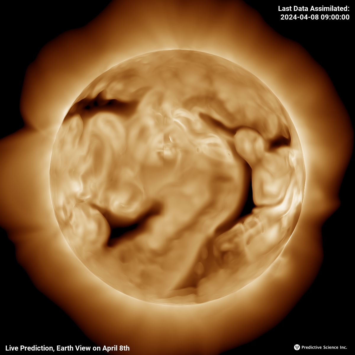
EUV 193Å Emission
(AIA)

Total Brightness
(K-Corona)
Br on the Sphere
(Surface Boundary Condition)
Volume Rendered Squashing Factor
(Emphasizing Low Corona)
EUV 193Å Emission
(AIA)
Coronal Brightness
Br on the Sphere
(Surface Boundary Condition)
Volume Rendered Squashing Factor
(Emphasizing Low Corona)
EUV 193Å Emission
(AIA)
Coronal Brightness
\(\def\npar {\partial}\)
The solar magnetic field \({\bf B}\) plays a key role in solar and heliospheric physics. On small scales, energy released from \({\bf B}\) heats the solar corona and accelerates the solar wind. At somewhat larger scales (e.g. active regions), energy stored in the magnetic field is at times violently released to power solar flares and coronal mass ejections. On global scales, \({\bf B}\) largely determines the topology and geometric features of the solar corona (e.g. coronal holes and streamers). It is this structure that partitions the solar wind into fast and slow streams, determines the location of the heliosphere current sheet (HCS), influences the propagation of coronal mass ejections (CMEs), and guides the propagation of solar energetic particles (SEPs). The solar \({\bf B}\) is therefore a crucial input to models of the solar corona.
This field is measured most reliably in the photosphere, with instruments such as the Helioseismic and Magnetic Imager (HMI) onboard NASA's Solar Dynamics Observatory (SDO), the Vector Spectromagnetograph (VSM), part of National Solar Observatory/Synoptic Optical Long-term Investigations of the Sun (NSO/SOLIS) and the NSO Global Oscillation Network Group (GONG) network.
Coronal MHD models using solar magnetic maps as boundary conditions have been used for many years to study the solar corona and inner heliosphere. The models are typically integrated to steady state for a given boundary map. In reality, the solar corona is constantly evolving in response to the changing photospheric \({\bf B}\). This is especially true during the most active years of the solar cycle, when the photospheric \({\bf B}\) is evolving rapidly.
What data do we need to drive a time-dependent model? Ideally, continuous observations of the Sun’s \({\bf B}\) observed over the entire surface, but these observations are not available. Instead, we use a surface flux transport model (HipFT) to ingest magnetograms and evolve the surface field where observations are not available. HipFT provides us with a sequence of maps specifying the photospheric B evolution. Lionello et al. (2023) describes our boundary driving technique. Here we note that in MHD models, the evolution of magnetic fields is specified via the tangential electric field at the boundary \({\mathbf E}_{t0}(\theta,\phi,t)\). In general, \({\mathbf E}_{t0}\) can be written in terms of two potentials \(\psi(\theta,\phi,t)\) and \(\mit\Phi(\theta,\phi,t)\) as \begin{equation} {\mathbf E}_{t0} = \nabla \times \psi \hat r + {\bf \nabla}_t {\mit\Phi}. \label{e-tangential} \end{equation} The potential \(\psi\) controls the evolution of the normal component of the magnetic field \(B_{r0}\), such that: \begin{equation} c{\nabla}^2_t \psi = \npar B_{r0} / \npar t. \label{eq-psi} \end{equation} We use a sequence of smoothed HipFT maps to specify the evolution of \(\psi\) using the above equations. The potential \(\mit\Phi(\theta,\phi,t)\) controls the change in the transverse components of the magnetic field. It can be completely specified if the flows that led to the evolution are known, i.e., we can find \(\mit\Phi\) from the equation: \begin{equation} c{\nabla}^2_t {\mit\Phi} = -\nabla_t\cdot(\mathbf{v} \times \mathbf{B})_t. \label{eq-phi} %\vspace{-.05in} \end{equation} From HipFT we only know some of the flows. In general, if we use only these flows, the coronal \({\bf B}\) will be under-energized, relative to the real Sun, because HipFT only provides \(B_{r0}\) and no information about the currents emerging with the fields. We use a potential \(\mit\Phi\) to energize the field, especially along polarity inversion lines. This is a generalization of the procedure we first used for the 2017 eclipse prediction.
Lionello et al. (2023) and Mason et al. (2023) describe the application of the method to a month of solar evolution. For that case, we used a sequence of maps from an idealized, Sun-like evolution. Here, for the first time, we employ the method to assimilate actual observations and drive a real time model of the solar corona.