Reconstructing Surfaces

This example demonstrates add_surface() — the method for building a triangulated surface through scattered spherical coordinate points using one of three reconstruction strategies: 'delaunay_2d', 'delaunay_3d', or 'reconstruct_surface'.

import numpy as np
from pyvisual import Plot3d

Surface of Revolution

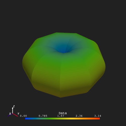
The surface below is defined by the relation \(r = 5\sin\theta\), sampled at 10 equally-spaced longitudes and 100 latitudinal points per meridian. The resulting point cloud forms a closed, non-planar surface that wraps around itself — the default 'delaunay_2d' projects points onto a plane before triangulating, which produces incorrect connectivity for such a surface. delaunay_3d() instead builds a full volumetric tetrahedralization and extracts the outer boundary, correctly handling the closed topology. The surface is colored by colatitude \(\theta\).

n_lines, n_pts = 10, 100
t = np.tile(np.linspace(0, np.pi, n_pts), (n_lines, 1))
r = 5 * np.sin(t)
p = np.tile(np.linspace(0, 2 * np.pi, n_lines)[:, None], (1, n_pts))

plotter = Plot3d(off_screen=True, window_size=(500, 500))
plotter.show_axes()
plotter.add_sun()
plotter.add_surface(r, t, p, t, method='delaunay_3d')
plotter.show()

Static Scene

Interactive Scene

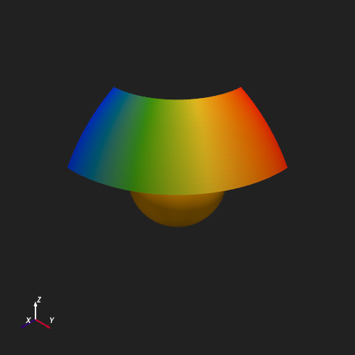
Open Shell Patch (delaunay_2d)

For nearly-planar or open surfaces, 'delaunay_2d' gives better results. The example below samples a spherical cap at \(r = 3\,R_\odot\) over a limited colatitude/longitude range and reconstructs it as a surface patch colored by longitude \(\phi\).

n_t, n_p = 20, 40
t_vals = np.tile(np.linspace(np.pi / 6, np.pi / 3, n_t), (n_p, 1)).T
p_vals = np.tile(np.linspace(0, np.pi / 2, n_p), (n_t, 1))
r_vals = np.full_like(t_vals, 3.0)

plotter = Plot3d(off_screen=True, window_size=(500, 500))
plotter.show_axes()
plotter.add_sun()
plotter.add_surface(r_vals, t_vals, p_vals, p_vals, method='delaunay_2d',
                    show_scalar_bar=False)
plotter.show()

Static Scene

Interactive Scene