Constructing a SphericalMesh

This example demonstrates how to build a SphericalMesh from NumPy arrays, inspect its properties, and add it to a Plot3d scene.

SphericalMesh wraps pyvista.RectilinearGrid with a spherical-frame tag. The three PSI spherical axes — radius \(r\), colatitude :math:` heta`, and longitude \(\phi\) — are stored as the x, y, and z axes of the rectilinear grid and aliased through the r, t, and p properties.

import numpy as np
from pyvisual import Plot3d
from pyvisual.core.mesh3d import SphericalMesh

Building from Axis Arrays

Pass three 1-D arrays (r, t, p) and an optional data array to construct the mesh. Here we build a dipole-like radial magnetic field \(B_r \approx \cos\theta / r^2\) on a coarse grid spanning the inner corona (\(r \in [1,\,10]\,R_\odot\)).

r = np.linspace(1, 10, 20)
t = np.linspace(0, np.pi, 30)
p = np.linspace(0, 2 * np.pi, 60)

R, T, P = np.meshgrid(r, t, p, indexing='ij')
Br = np.cos(T) / R ** 2

mesh = SphericalMesh(r, t, p, data=Br, dataid='Br')

print(f"dimensions : {mesh.dimensions}")
print(f"r range    : [{mesh.r.min():.1f}, {mesh.r.max():.1f}] R_sun")
print(f"t range    : [{mesh.t.min():.3f}, {mesh.t.max():.3f}] rad")
print(f"p range    : [{mesh.p.min():.3f}, {mesh.p.max():.3f}] rad")
print(f"data range : [{mesh.data.min():.3f}, {mesh.data.max():.3f}]")

dimensions : (20, 30, 60)
r range    : [1.0, 10.0] R_sun
t range    : [0.000, 3.142] rad
p range    : [0.000, 6.283] rad
data range : [-1.000, 1.000]

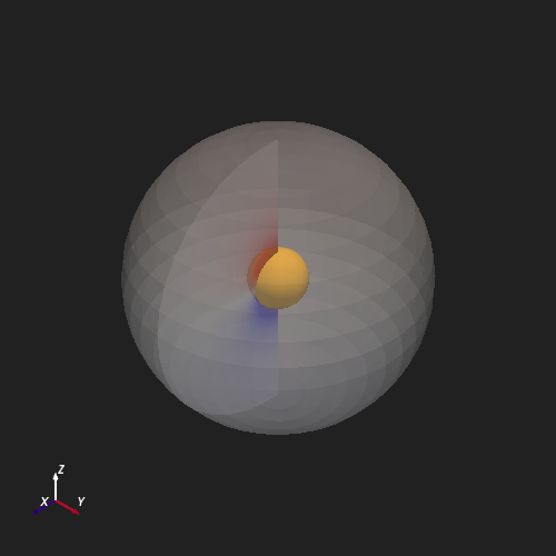
Adding to a Plot3d Scene

Plot3d reads the MESH_FRAME key from the mesh’s user_dict and automatically converts the spherical coordinates to Cartesian before rendering — no explicit frame argument is required.

plotter = Plot3d(off_screen=True, window_size=(500, 500))
plotter.show_axes()
plotter.add_sun()
plotter.add_mesh(mesh, cmap='seismic', clim=(-0.5, 0.5), opacity=0.4)
plotter.show()

Static Scene

Interactive Scene

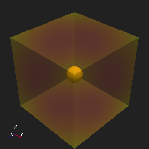
Slicing the Mesh

SphericalMesh supports standard NumPy-style index slicing on its spatial axes. The result is a new SphericalMesh containing the sliced coordinate arrays and the corresponding data subset. Here we extract the innermost 5 radial shells.

sub = mesh[0:5, ...]
print(f"sliced dimensions : {sub.dimensions}")

plotter = Plot3d(off_screen=True, window_size=(500, 500))
plotter.show_axes()
plotter.add_sun()
plotter.add_mesh(sub, cmap='seismic', clim=(-0.5, 0.5), opacity=0.6)
plotter.show()

Static Scene

Interactive Scene

sliced dimensions : (5, 30, 60)