Observer Position and Focus

This example demonstrates the observer_position and observer_focus properties — the primary interface for positioning the camera in spherical coordinates.

Both properties accept and return spherical coordinates \((r, heta, \phi)\) where :math:` heta` is the colatitude (measured from solar north) and \(\phi\) is the longitude. Setting either property immediately re-renders the scene.

import numpy as np
from pyvisual import Plot3d

Positioning the Observer

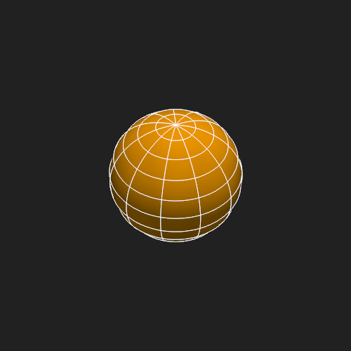
The default camera position is set by PyVista’s auto-fitting algorithm. observer_position lets you override it with a specific \((r, \theta, \phi)\) location. Here the observer is placed at \(r = 10\,R_\odot\), \(\theta = \pi/4\) (45° from the north pole), and \(\phi = \pi/4\) (45° longitude).

plotter = Plot3d(off_screen=True, window_size=(500, 500))
plotter.add_sun()
plotter.add_longlat_lines()
plotter.observer_position = 10, np.pi / 4, np.pi / 4
plotter.show()

Static Scene

Interactive Scene

Equatorial View

Moving the observer to the equatorial plane (\(\theta = \pi/2\)) gives a side-on view of the solar equator — a perspective typical of coronagraph imagery from an ecliptic observer.

plotter = Plot3d(off_screen=True, window_size=(500, 500))
plotter.add_sun()
plotter.add_longlat_lines()
plotter.observer_position = 10, np.pi / 2, 0
plotter.show()

Static Scene

Interactive Scene

Reading Back the Observer State

The getter returns a SphericalCoordinate named tuple, providing field-name access to r, t, and p.

plotter = Plot3d(off_screen=True, window_size=(500, 500))
plotter.add_sun()
plotter.add_longlat_lines()
plotter.observer_position = 10, np.pi / 2, 0
pos = plotter.observer_position
print(f"r = {pos.r:.2f} R_sun")
print(f"t = {pos.t:.4f} rad  ({np.rad2deg(pos.t):.1f} deg colatitude)")
print(f"p = {pos.p:.4f} rad  ({np.rad2deg(pos.p):.1f} deg longitude)")
plotter.show()

Static Scene

Interactive Scene

r = 10.00 R_sun
t = 1.5708 rad  (90.0 deg colatitude)
p = 0.0000 rad  (0.0 deg longitude)