Field-of-View Controls

This example demonstrates two complementary properties for controlling the observer’s field of view (FOV):

• observer_los_view — specify the FOV as explicit helioprojective angular extents (x0, x1, y0, y1) in degrees.

• observer_fov_view — specify the FOV by the minimum line-of-sight impact radius \(r_\mathrm{min}\) in \(R_\odot\).

Both setters update the camera’s view angle and focal point simultaneously. observer_position must be set before either FOV property, because the focal-point calculation depends on the observer distance.

from math import pi
from pyvisual import Plot3d

Coronagraph View via Angular Extents

observer_los_view accepts a 4-tuple (x0, x1, y0, y1) of helioprojective angular extents in degrees. Here we simulate a coronagraph at \(r = 50\,R_\odot\) on the equatorial plane with a \(\pm 10°\) horizontal by \(\pm 8°\) vertical FOV centered on the Sun.

plotter = Plot3d(off_screen=True, window_size=(500, 500))
plotter.add_sun()
plotter.add_longlat_lines()
plotter.observer_position = 50, pi / 2, 0
plotter.observer_los_view = -10, 10, -8, 8
plotter.show()

Static Scene

Interactive Scene

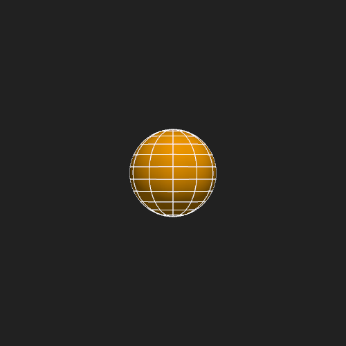
Coronagraph View via Impact Radius

observer_fov_view expresses the FOV in physical units: the setter computes the symmetric half-angle \(\alpha = \arcsin(r_\mathrm{min} / d_\mathrm{obs})\) and forwards it to observer_los_view as \((-\alpha, +\alpha, -\alpha, +\alpha)\).

Setting \(r_\mathrm{min} = 4\,R_\odot\) sizes the FOV so that the outermost lines of sight just graze the corona at 4 solar radii — a natural choice for an instrument designed to observe mid-corona dynamics.

plotter = Plot3d(off_screen=True, window_size=(500, 500))
plotter.add_sun()
plotter.add_longlat_lines()
plotter.observer_position = 50, pi / 2, 0
plotter.observer_fov_view = 4
plotter.show()

Static Scene

Interactive Scene