Example 1.3: Scaled Slices

Shortcuts are written Ctrl+…; macOS shows ⌘.

Goal

Cut the same file along theta and phi, and apply two kinds of scaling: scaling the data and scaling a scale.

Index versus value windows

Example 1.2 used index windows, which count grid points and change meaning if the grid is regridded. A value window, such as t of {value: [90, 90], unit: deg} for the equator, is physical and survives a change of resolution. An equal pair selects one coordinate, interpolated to that value. Setting Read’s method to value enables value windows. This example keeps index windows for simplicity.

Functions: unary and binary

Functions (the Functions menu) take datasets and return datasets. A unary function has one input, x, and a target that selects which arrays it acts on (the data, or a scale such as scale_r). A binary function has two inputs, a and b, as in Multiply, where a is the data and b the factor. Some binary functions, such as Power, make b optional: a fixed field (exponent) stands in when nothing is connected.

Scaling the data versus scaling a scale

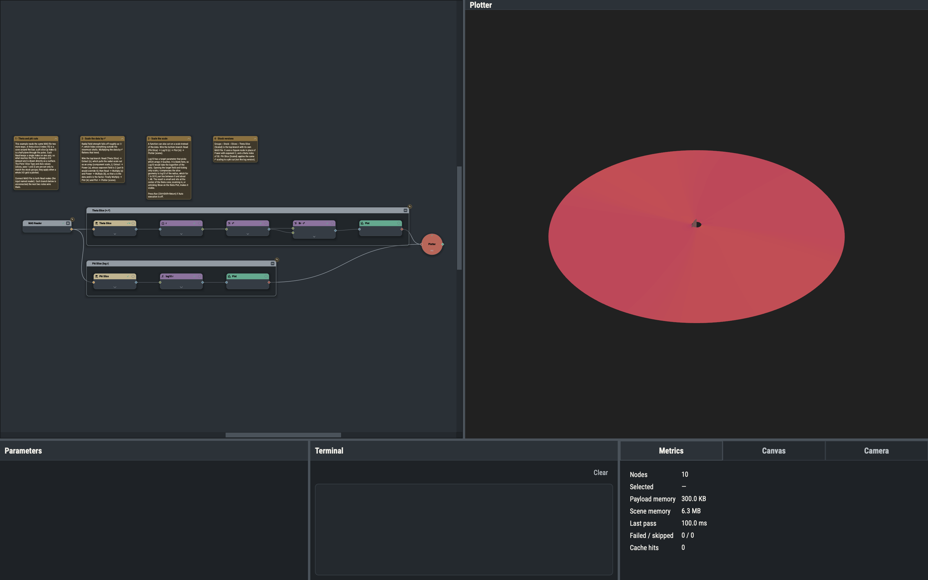
Multiplying Br by r² changes the values: the radial falloff is removed and structure far from the Sun becomes visible. Extract pulls the radial scale out as an array, which is raised to the power 2 and used as the factor.

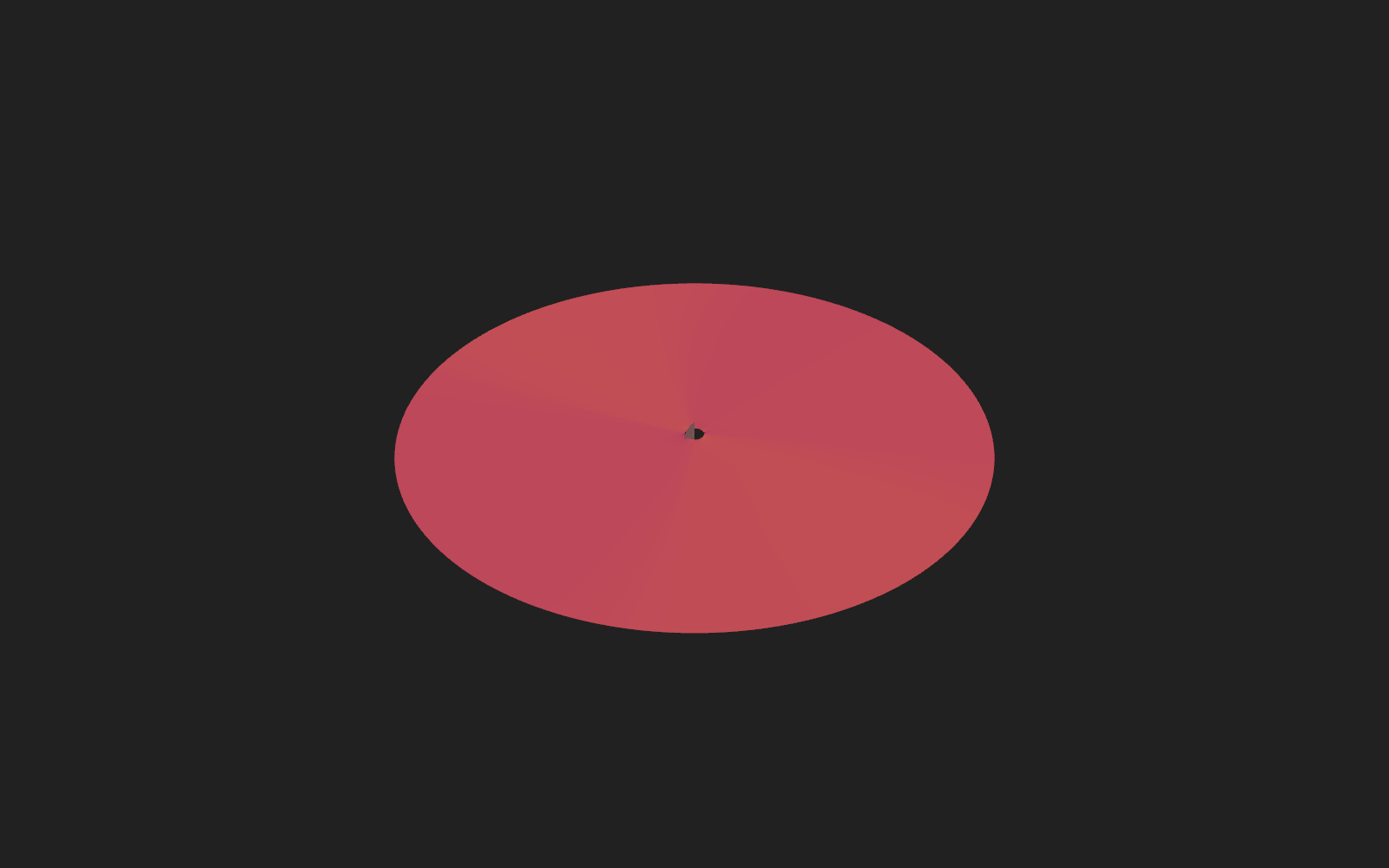
Log10 with target: [scale_r] changes the geometry instead. Only the radial axis is replaced by its base-10 logarithm, so a slice that spans 1 to 30 R_sun is drawn between 0 and about 1.48. The data is untouched.

Set Scale

Set Scale replaces the scale of one axis. With its value field, the axis must have length one (a single radial cut, or the placeholder radial axis of a 2-D map); an array connected to the optional scale port replaces an axis of any length when the lengths match. Example 1.4 uses it to give a 2-D map a radius.

Variations

• An Offset node (Functions ▸ Unary ▸ Misc, offset 1, target scale_r) after Log10 lifts the slice off the origin.
• Setting Power’s exponent to 0.5 or 1 gives a different scaling.
• Setting Read’s method to value and cutting at phi = 0 degrees selects the slice by physical position instead of by index.

Example 1.4 draws a 2-D map on the solar surface.