 PVA
Example 1.4: The Coronal Hole Map
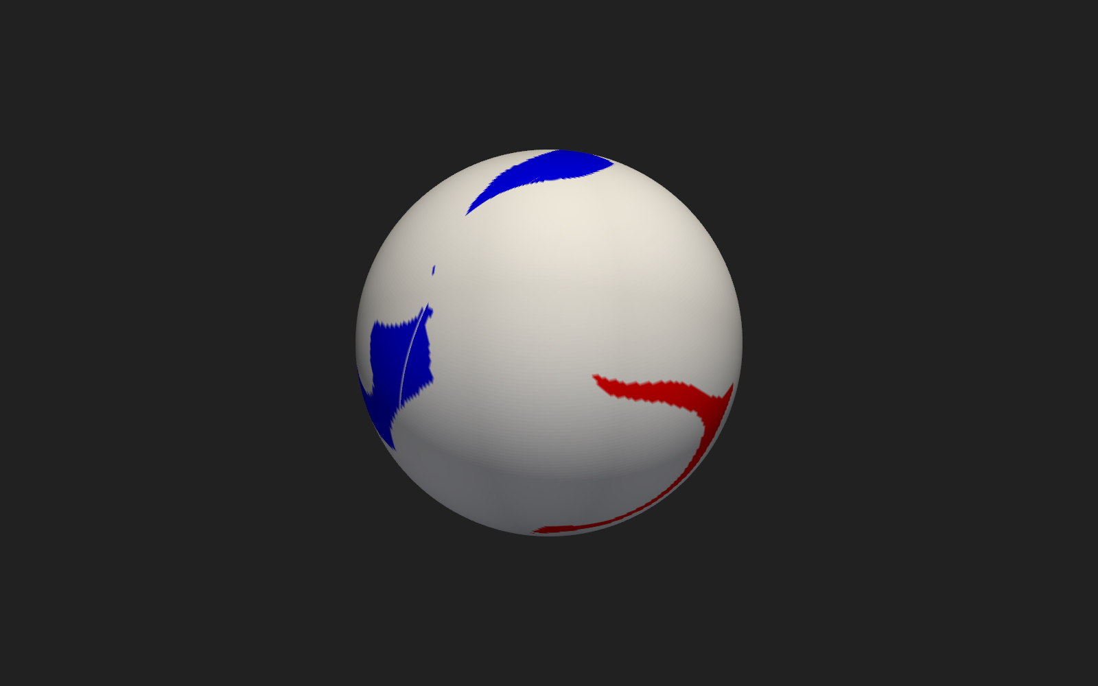
Draw a 2-D map of the Sun's surface by giving it a radius.
Shortcuts are written Ctrl+…; macOS shows ⌘.
Goal
Draw a 2-D map of the Sun’s surface by giving it a radius.
2-D datasets and the Plot rows
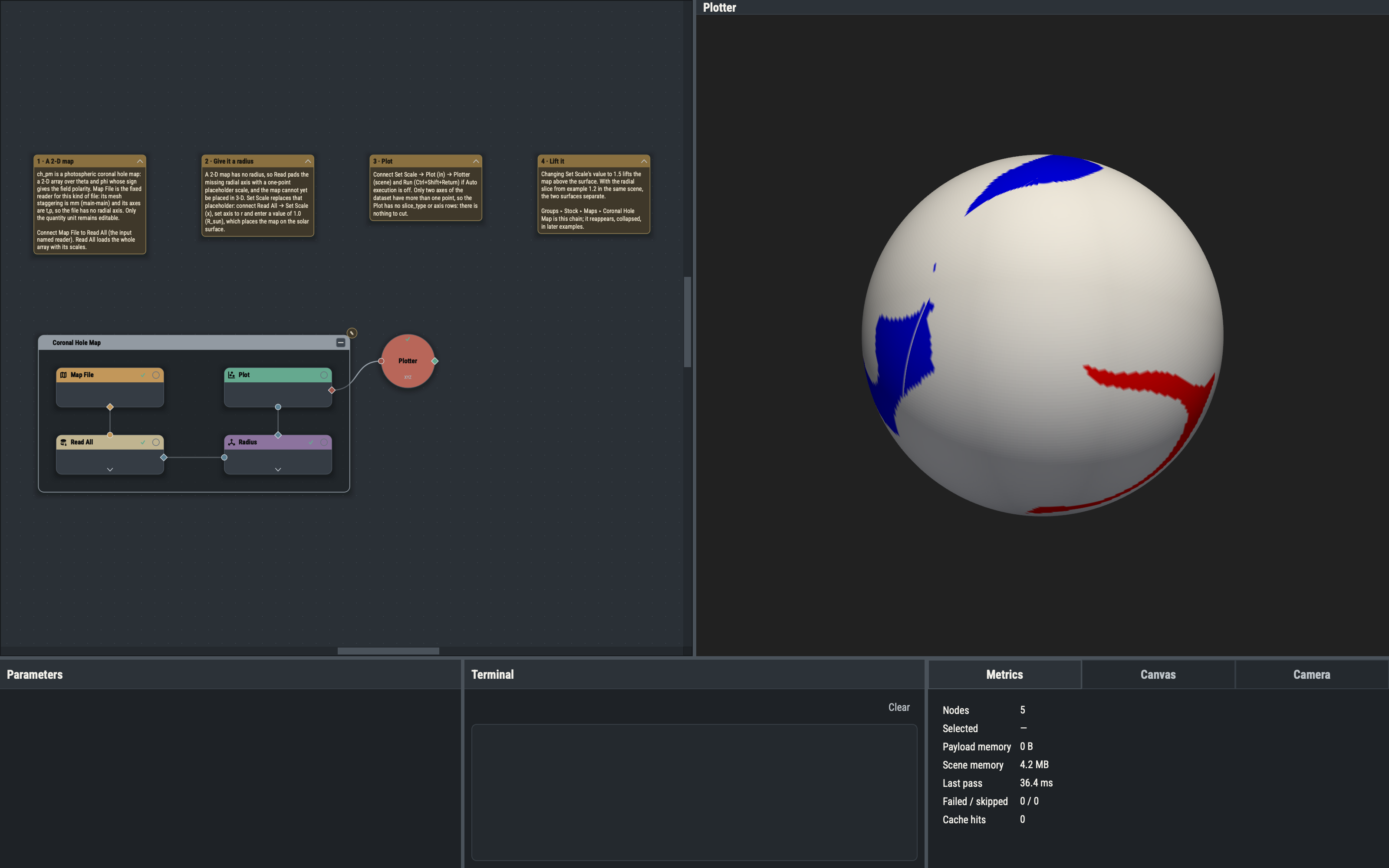
The ch_pm sample is a polarity map over theta and phi. A dataset with only two non-singleton axes has nothing to slice, so the Plot node hides slice_type and axis and draws the surface directly.
Map File versus MAS File
MAS File reads 3-D model output and carries model metadata (variable, unit, mesh). Map File is a fixed 2-D reader: its mesh staggering is mm (main-main) and its axes are t,p, so it is always interpreted as a (theta, phi) map. Only the quantity unit is editable.
Set Scale on a singleton axis
Read pads the axes missing from a 2-D file with a one-point placeholder scale, so Read All loads the array with its scales but no meaningful radius. Set Scale replaces the placeholder radial scale with the given value. A value of 1.0 R_sun places the map on the solar surface; larger values lift it onto a shell, which allows comparison with a quantity defined at a different height.
Variations
- With the example 1.2 Radial Slice group wired to the same Plotter, a Set Scale value of 1.5 lifts the map clear of the slice.
- Lowering the Plot’s
opacitymakes the map translucent.
Example 2.1 traces magnetic field lines. The Coronal Hole Map appears in later examples as a collapsed group for context.