Example 2.1: Field-Line Tracing

Shortcuts are written Ctrl+…; macOS shows ⌘.

Goal

Trace magnetic field lines through the corona in three ways, and color them by length and by polarity.

What a Tracer is

A Tracer is a generator that wraps mapflpy, the Python interface to the MAS field-line tracer. Given the three field components (br, bt, bp) it holds the field in a background process. Trace nodes ask it for lines; the Tracer does no work until they do.

Direction

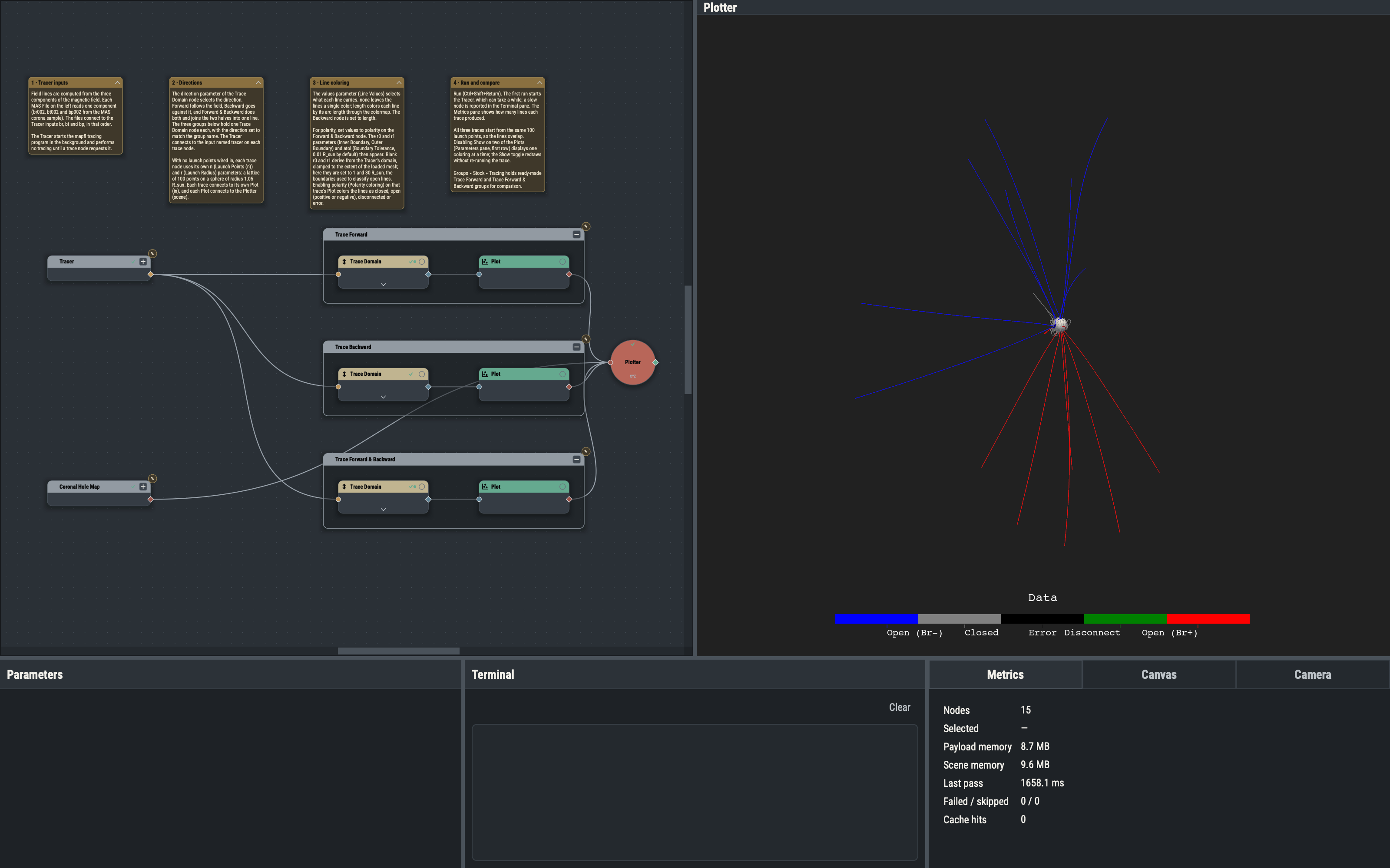
One node, Trace Domain, does all three. Its direction parameter (Direction) chooses Forward, which follows the field vector, Backward, which goes against it, or Forward & Backward (the default), which does both and joins the halves into one line through the launch point.

Launch points

With nothing wired into lps, a trace uses its own n and r parameters: a deterministic Fibonacci lattice of n points (100 by default) on a sphere of radius r (1.05 R_sun by default, just above the surface). Example 2.2 replaces this with supplied points.

Line values and coloring

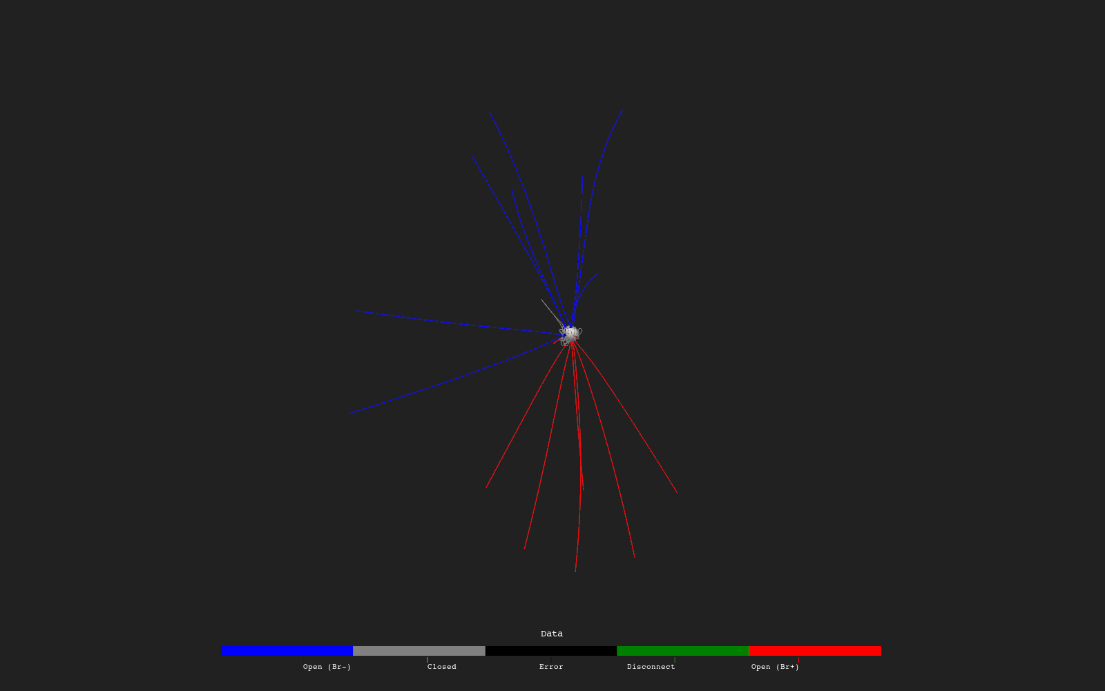
values decides what each line carries: none (nothing, so a single color), length (arc length) or polarity. Polarity classifies each line as closed, open with positive or negative sign, disconnected, or error (a line that failed to reach a boundary). A Plot of field lines uses form: splines with fieldlines on; tick polarity on the Plot to color by that classification.

Boundaries r0, r1 and atol

Polarity classification requires the radii where lines end. r0 is the inner boundary (Inner Boundary), r1 the outer (Outer Boundary), and atol (Boundary Tolerance, 0.01 R_sun by default) the tolerance for counting a line as having reached one. These three parameters are shown only while values is polarity. Blank r0 and r1 take derived defaults: the Tracer’s domain radii, clamped to the extent of the loaded mesh (r0 is the larger of the domain minimum and the mesh minimum, r1 the smaller of the domain maximum and the mesh maximum). The tutorial sets them explicitly (1 and 30 R_sun) so the result does not depend on the data.

Why axis 1 on fieldline Plots

For line stacks, axis names the array axis that runs along each line. Field lines are stored as (lines, points per line), so axis: 1 joins each line’s own points into a curve; axis: 0 would join the n-th point of every line into an incorrect curve.

Tracer timeout

Tracing can be slow. A trace fails when the Tracer subprocess does not answer within the subprocess timeout, set in Settings… (File menu, or the PVA app menu on macOS; Ctrl+,) ▸ Defaults ▸ Tracer ▸ Subprocess timeout (60 s by default).

Variations

• Setting n to 300 on one trace launches 300 lines instead of 100.
• Setting r to 1.5 launches the lines from a higher sphere.
• Raising Max Steps / Line (buffer_size, 2000 by default) on a trace node allows longer lines before the step buffer is exhausted.

The scalar bar is per Plot: the length-colored Plot hides its bar so that it does not overlap the polarity bar. All three traces start from the same launch points, so the lines overlap; disabling Show on a Plot displays one coloring at a time.

Example 2.2 covers supplying launch points.