 PVA
Example 3.1: Spacecraft Ephemeris
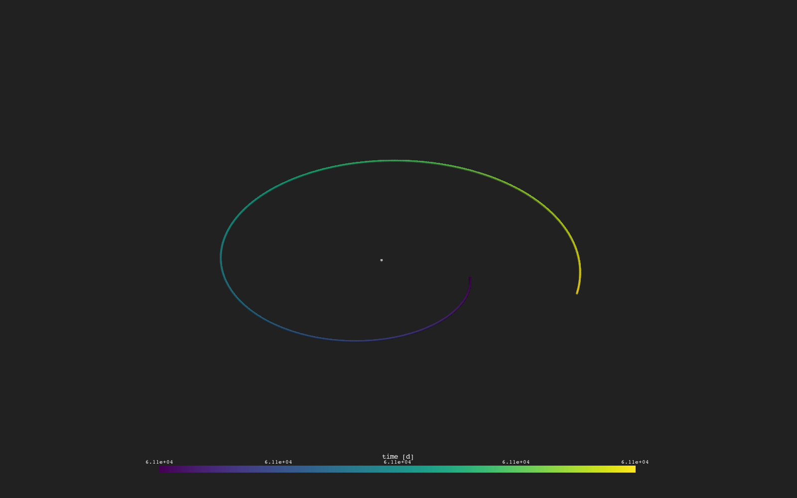
Fetch a spacecraft's trajectory for a chosen time window and plot it around the Sun.
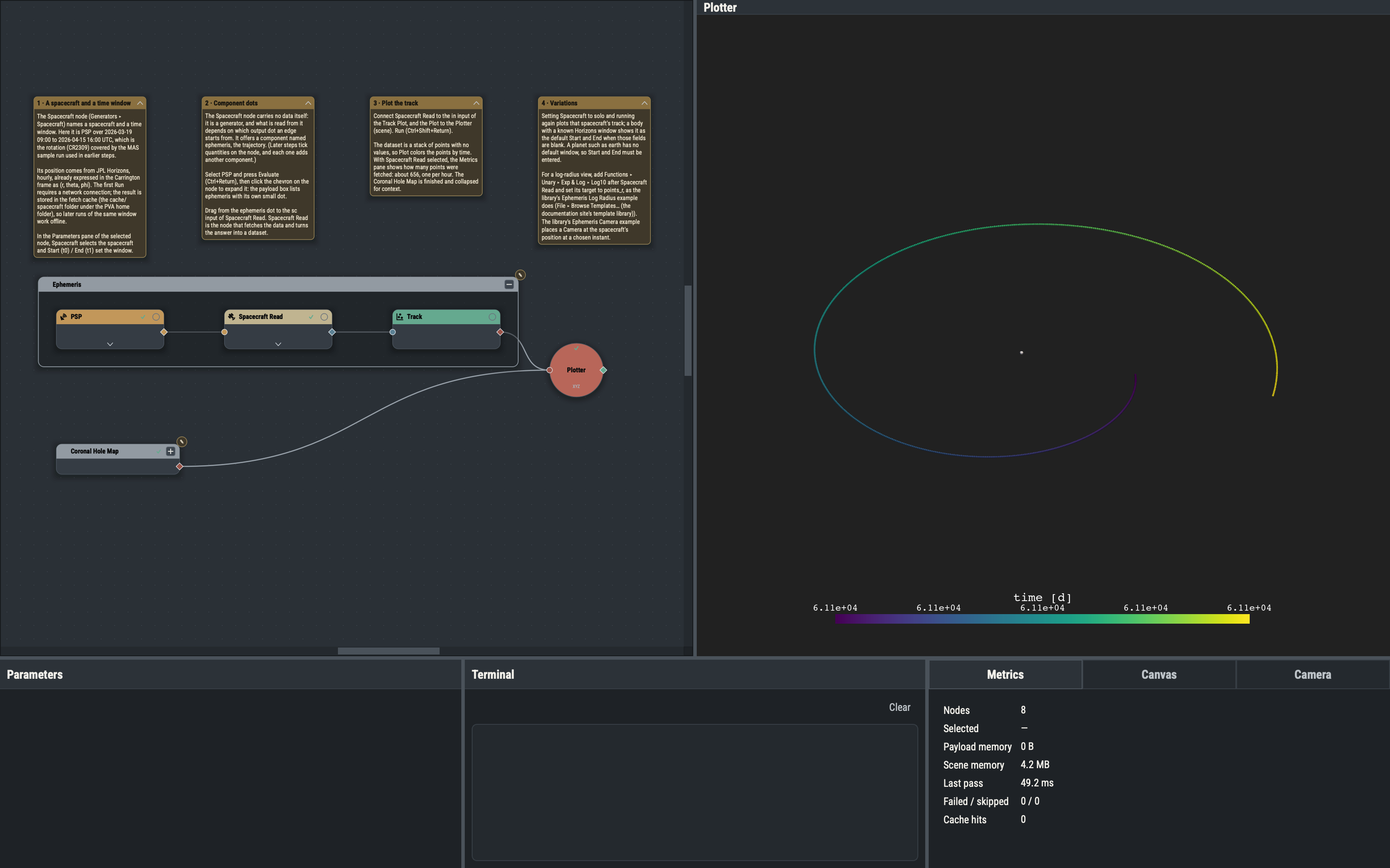
Shortcuts are written Ctrl+…; macOS shows ⌘.
Goal
Fetch a spacecraft’s trajectory for a chosen time window and plot it around the Sun.
Where the data comes from
The Spacecraft node requests the position of the selected spacecraft from JPL Horizons (through the sunpy package). The answer is hourly and is already converted to the Carrington frame, so each point is (r, theta, phi) with r in R_sun and the angles in radians, the same frame as the MAS model data. The time window used here is the CR2309 rotation that the MAS sample run covers, so the track and the model line up in time.
The first Run requires a network connection. The result is saved in the fetch cache, the cache/spacecraft folder under the PVA home folder (Spacecraft Read has a Use Fetch Cache switch), so running the same window again works offline. If the network is unavailable and the window is not cached, the node reports an error in the Terminal pane and nothing is drawn.
Generators with component dots
Spacecraft is a generator, like a MAS File: it describes what can be read rather than holding the data. A generator can offer several things at once, and each one is an output dot of its own, called a component dot. Spacecraft always offers ephemeris; example 3.2 adds one dot per in situ quantity. An edge from a component dot records which one it carries, which determines what Spacecraft Read fetches.
Stack datasets and the time scale
Spacecraft Read returns a stack dataset: an ordered list of points rather than a grid. It has r, theta and phi coordinates for every point, a time scale (the time of each point, in days) and, for in situ data, value arrays. A stack with no value arrays is colored by its time scale, so the Plot shows a color bar labeled time.
Sampling modes
The Sampling parameter on the Spacecraft node controls which times are returned. Each requested time is snapped to the nearest hourly row:
all: every hourly point between Start (t0) and End (t1).linspace:nevenly spaced times in the window.geomspace:ntimes spaced geometrically, dense near the start.explicit: a list of times typed into the Times field. Start and End are hidden in this mode.
Variations
- Setting Spacecraft to
soloand adjusting the window to dates that spacecraft covers changes the track. A body with a known Horizons window (for examplepsporsolo) shows that window as the default Start and End; a planet such asearthhas no default window, so Start and End must be entered. - Setting
sampling: linspacewithn: 24returns a thinned track of 24 points. - A Log10 with
target: points_rafter Spacecraft Read compresses the radial range (the Ephemeris Log Radius template in the library, File ▸ Browse Templates…, does this). - The Ephemeris Camera template in the library (File ▸ Browse Templates…) places a Camera at the spacecraft’s position.
Example 3.2 covers reading measurements taken along the track and comparing them with the model.