Example 3.2: In Situ Data Versus the Model

Shortcuts are written Ctrl+…; macOS shows ⌘.

Goal

Plot the magnetic field a spacecraft measured along its track, then sample the MAS model at the same points and compare the two in separate viewports.

HAPI, CDAWeb and the quantity list

For spacecraft that publish their measurements through the HAPI protocol, such as PSP, the Spacecraft node fetches in situ data from the CDAWeb archive. The In-situ quantities card lists what is available: br, bt, bp, flow_speed, rho, t, vr, vt and vp. The card is shown only for spacecraft that have an in situ archive. Fields are in Gauss, speeds in km/s, density in cm⁻³ and temperature in MK. Each ticked quantity adds its own component dot to the node, and the data are matched to the ephemeris times so every point has a position and a value. As in example 3.1, the first Run requires a network connection and the result is cached.

Spacecraft Read selects what to read from the component the edge carries: the ephemeris dot gives positions only; the br dot gives the same positions together with the br values.

Read method: points and the lps port

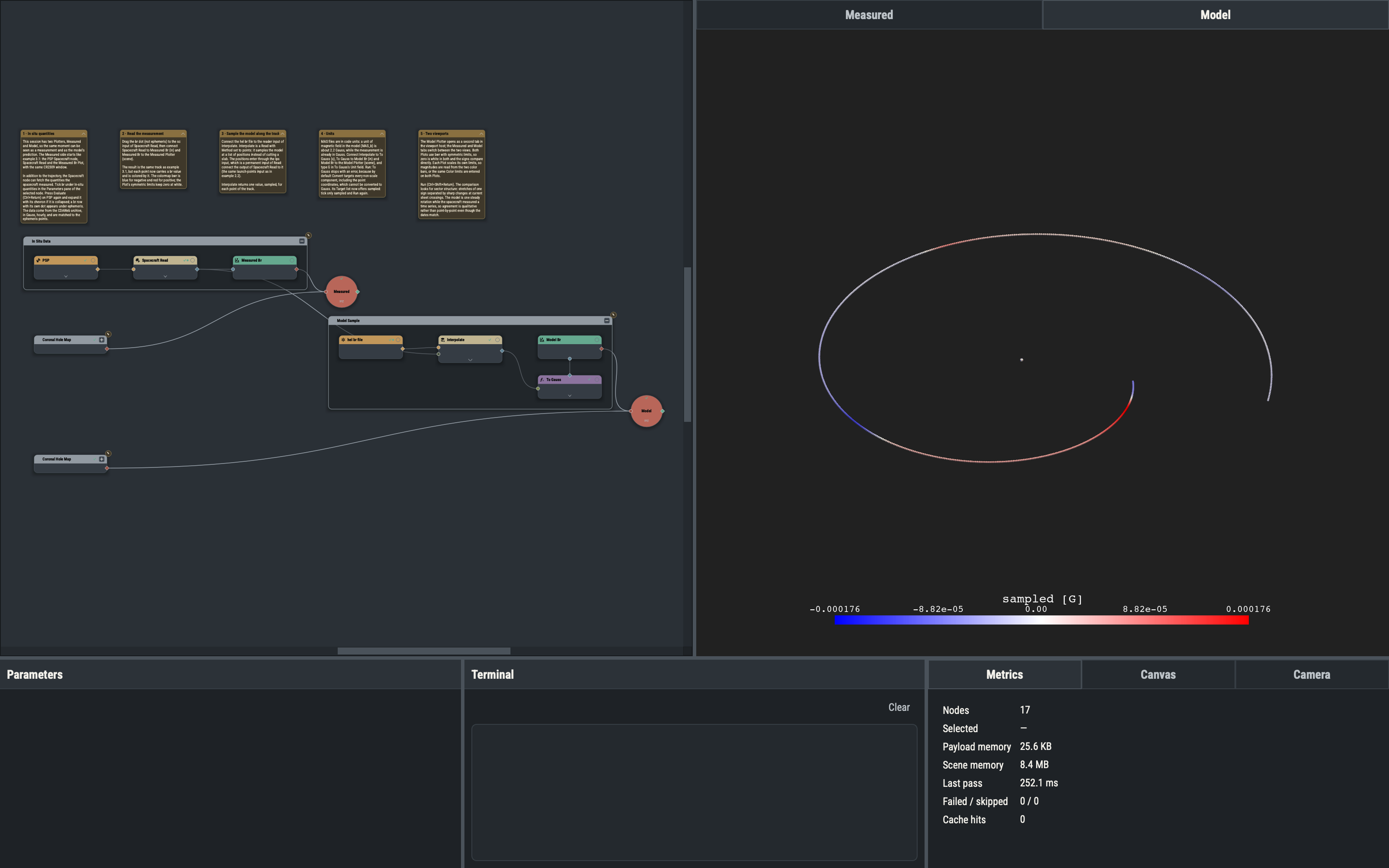
A Read with Method set to points does not cut a slab out of the model: it interpolates the model at a list of positions and returns the positions’ own dataset with the sampled array, named sampled, placed first: a stack stays a stack (field lines stay field lines, a grid stays a grid), keeping the arrays it already carries. Points that are NaN in the input stay NaN. The positions enter through the lps input, which is a permanent input port of the Read node. Here the positions are the track points from Spacecraft Read, so the model is sampled exactly where the spacecraft was. The positions use the same Carrington frame and units on both sides, so no conversion is needed.

Unit conversion and MAS code units

MAS files are stored in code units; for the magnetic field one unit (MAS_b) is about 2.2 Gauss. The Convert node (Functions ▸ Unary ▸ Convert) re-expresses values in another unit. A stack exposes its point coordinates as components too, and by default Convert targets every non-scale component, including the points, which cannot be converted to Gauss, so the first Run stops with an error. Once the node is wired and its input has been evaluated, its Target list offers sampled; ticking only that component and running again succeeds.

Extra plotters and viewport tabs

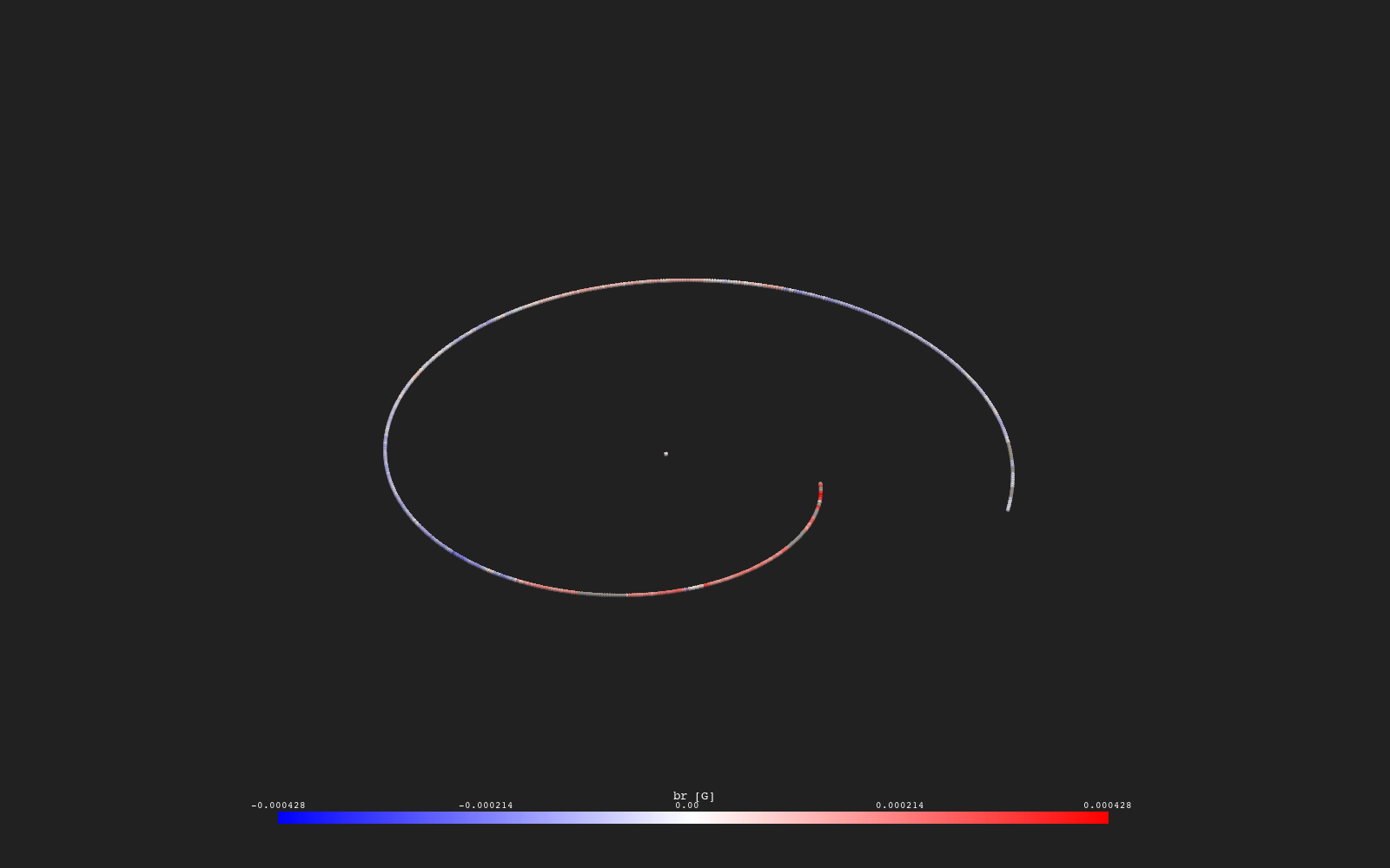
A second XYZ Plotter opens as a tab in the viewport host next to the main one. Plots wired to a Plotter appear only in that Plotter, so each tab can show a different view of the data. The Plotters here are named Measured and Model. Both Plots use the bwr colormap with symmetric limits, so zero is white in both and the signs compare directly. Each Plot scales its own limits, so magnitudes are read from the two color bars, or the same Color limits are entered on both Plots.

Interpreting the comparison

The model is one steady, synoptic snapshot of the corona and heliosphere for the rotation, while the spacecraft measured a time series that includes transients the model does not contain. Agreement is therefore qualitative: the comparison looks for the same sector structure (alternating signs of Br) and the position of the sign changes, not for matching values. Differences in magnitude are expected as well.

Variations

• Ticking flow_speed in Spacecraft and sampling the heliosphere vr002 file instead of br002, with Convert set to km/s, compares the measured and modeled flow speed.
• Setting Time Mode to window on Spacecraft Read and choosing a Start and End restricts the track to a shorter stretch.

Example 3.3 covers using the ephemeris as launch points for field line tracing.