 PVA
Example 3.3: Tracing from Spacecraft Positions
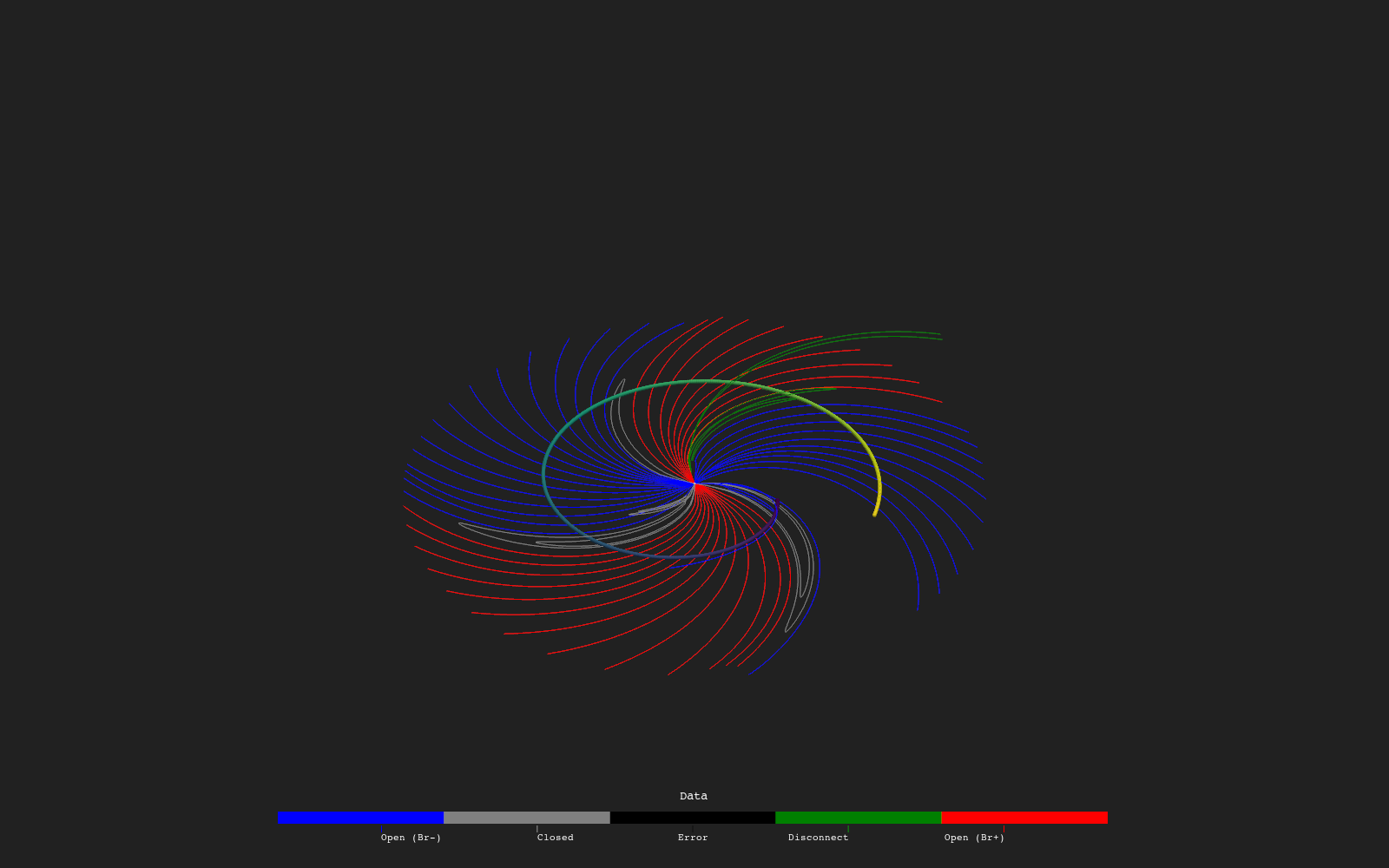
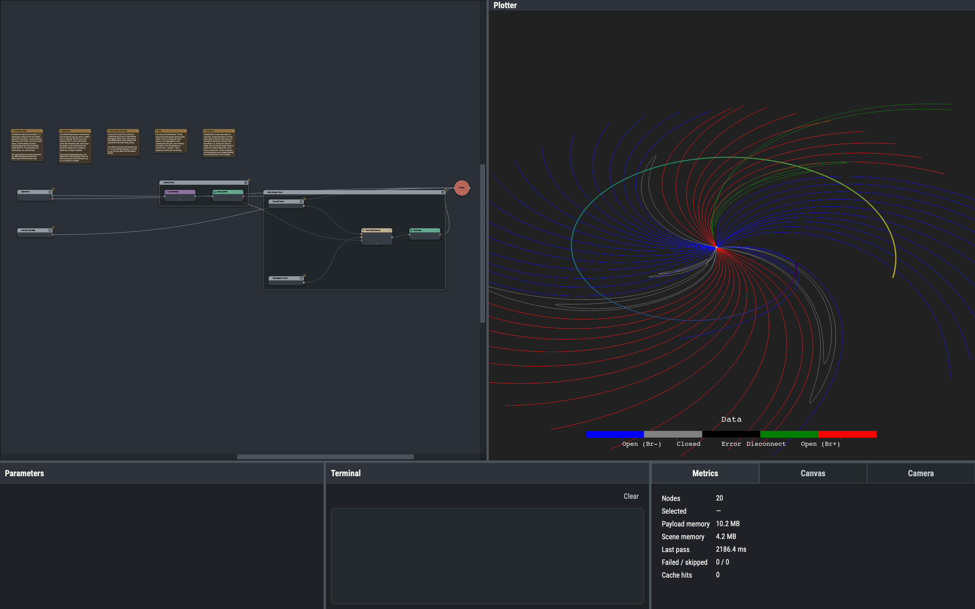
Start field lines from points along a spacecraft's track and trace each one through the corona and the heliosphere, using Trace Multi Domain to continue each line from one model domain into the other.
Shortcuts are written Ctrl+…; macOS shows ⌘.
Goal
Start field lines from points along a spacecraft’s track and trace each one through the corona and the heliosphere, using Trace Multi Domain to continue each line from one model domain into the other.
Why two models
MAS runs two grids: a corona domain out to about 30 R_sun and a heliosphere domain from 30 R_sun to 236 R_sun, each with its own files. A single Tracer holds only one domain, so a line that leaves it must be continued by the other. The handoff happens at the interface radius.
Why thin the track
The hourly ephemeris from example 3.1 has about 656 points for this window. Tracing that many lines is slow, and the picture is a solid mass of lines. The Downsample node (Functions ▸ Dataset) in stride mode keeps every stride-th point of a stack; with a stride of 12 about 55 points remain, one every half day, which is enough to show how the field the spacecraft crosses connects back to the Sun. On a grid dataset, Downsample uses stride_r, stride_t and stride_p instead.
Ephemeris points as lps
A stack of points can be wired straight into a trace node’s optional lps port (example 2.2), whatever generated it. The ephemeris from Spacecraft Read holds r, theta and phi in the Carrington frame, which is also the frame the tracers expect, so no frame conversion is needed. Each point becomes one launch point; the trace ignores its own n and r once lps is linked.
Trace Multi Domain parameters
r_interface(Interface Radius): the interface radius (30 R_sun by default).maxiter(Max Recross Iterations): how many times a line may be re-crossed between the domains before the trace gives up (10 by default).atol(Boundary Tolerance): the boundary tolerance (0.01 R_sun by default; 1 R_sun here).helio_shift(Heliospheric Phi Shift): a phi shift applied to the heliospheric domain (0 by default; degrees or radians).rtol(Interface Tolerance): the tolerance for matching positions at the interface (1e-5 by default).r0andr1: inner boundary (1 R_sun) and outer boundary (236 R_sun). When blank,r0derives from the coronal Tracer’s inner boundary andr1from the heliospheric Tracer’s outer boundary.
The shared trace parameters (n, r, buffer_size, values, the lps port) are the same as on the single-domain trace nodes.
Nested groups
The solved file nests the two Tracer groups inside the Inter-Domain Trace group, so the whole inter-domain trace collapses to a single card. Collapsing the outer group hides all of its members, and the inner groups can be collapsed independently.
Corotation caveat and helio_shift
The Carrington frame rotates with the Sun, and the MAS model is a steady solution in that frame, so a point at a given (r, theta, phi) means the same place in the model whatever time the spacecraft was there. The model does not evolve over the 27 days of the track, however, so the traced lines show the connectivity of the modeled rotation, not the field at each moment.
Changing helio_shift slides the heliospheric domain relative to the coronal one before the lines are handed across at the interface.
Variations
- Setting Downsample’s
strideto 6 or 24 changes the number of lines accordingly (about twice as many for 6, about half as many for 24). - Setting Line Values to
lengthon Trace Multi Domain colors the lines by length instead of polarity. - A different
helio_shiftchanges where the lines cross the interface. - The Spacecraft Launch Points template in the library (File ▸ Browse Templates…) is the finished version of this example.
- Connecting the Fibonacci Sphere from example 2.2 to the exposed
lpsport seeds the trace from those points instead of then/rlattice.
Example 3.4 draws a curtain of samples under a spacecraft’s orbit.