 PVA
Example 3.4: A Curtain Under the Orbit
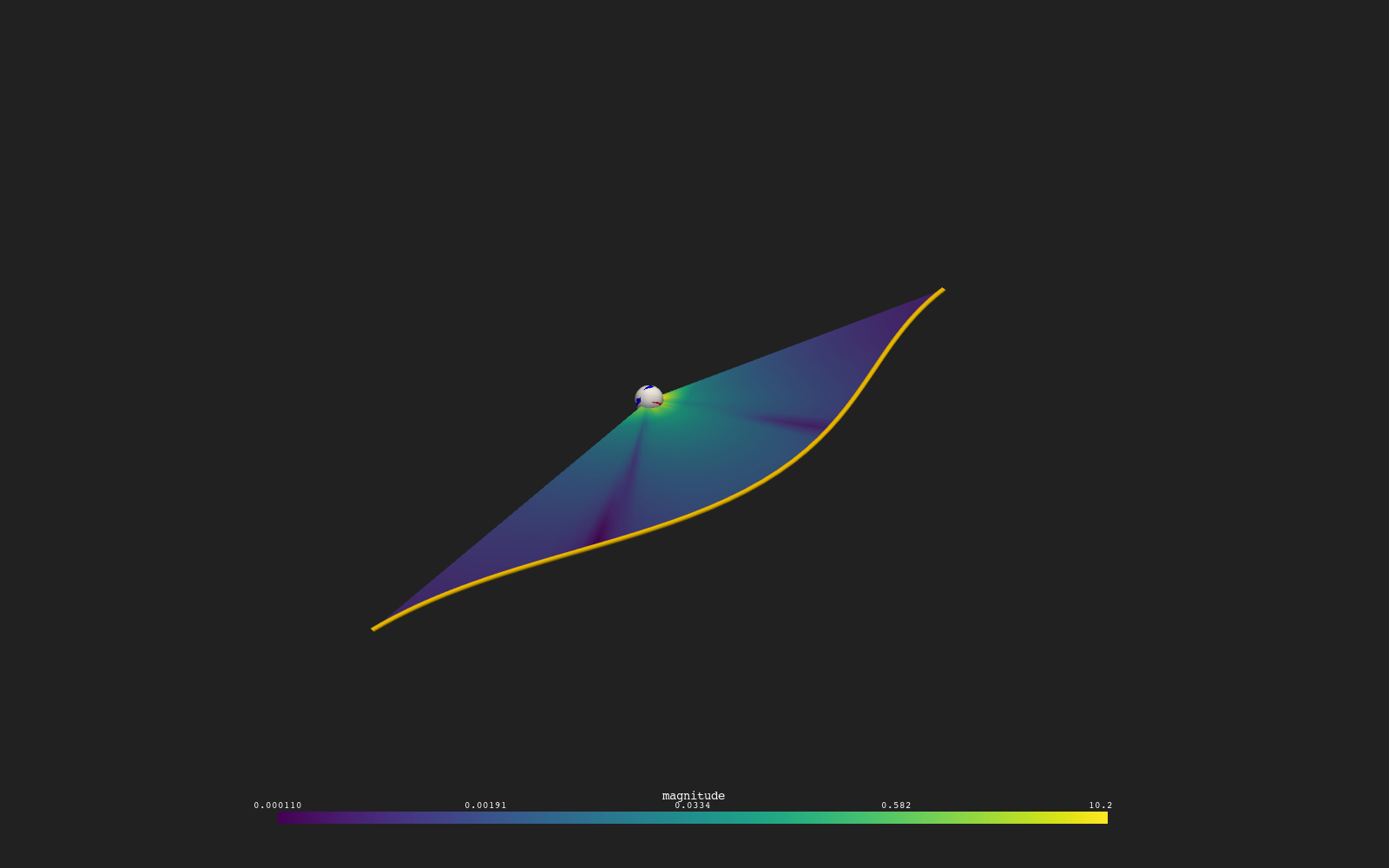
Hang a surface from a spacecraft's orbit down toward the Sun and color it with the magnitude of the model's magnetic field, sampled from three scalar files combined into a vector field.
Shortcuts are written Ctrl+…; macOS shows ⌘.
Goal
Hang a surface from a spacecraft’s orbit down toward the Sun and color it with the magnitude of the model’s magnetic field, sampled from three scalar files combined into a vector field.
The window and the data
The spacecraft is PSP, over 2024-03-28 to 2024-04-01 with 48 points spread evenly in time (Sampling linspace). This window differs from the CR2309 window of examples 3.1 to 3.3 on purpose: the public sample run covers the corona domain only to about 30 R_sun, and over these four days around perihelion PSP stays between about 11 and 29 R_sun, so every point of the curtain lies inside the data. The first Run needs a network connection for the positions (the same JPL Horizons request as in example 3.1); they are cached afterwards.
Curtain
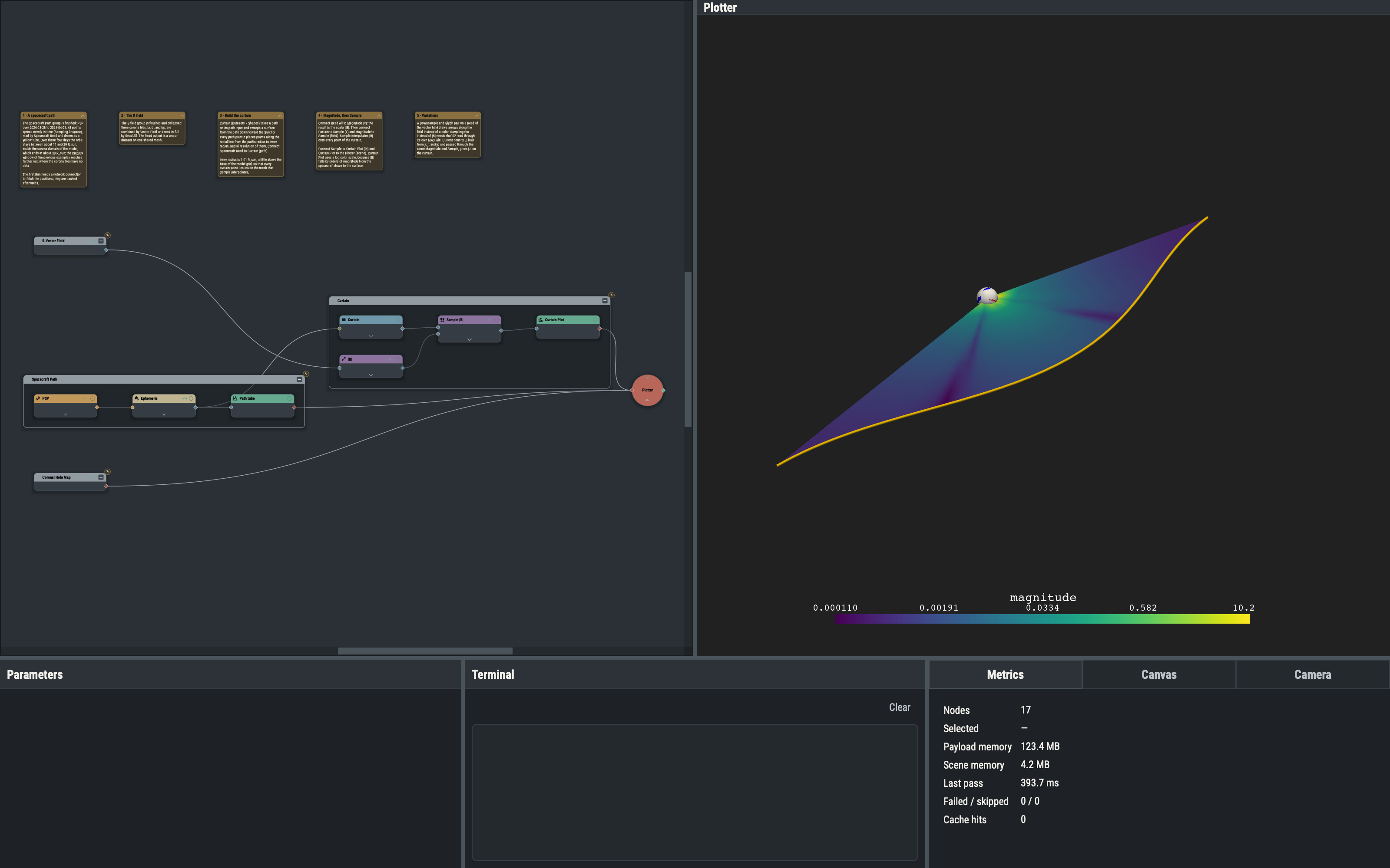
Curtain (Datasets ▸ Shapes) takes an ordered set of points on its path input, here the ephemeris from Spacecraft Read, and builds a ribbon: every path point is joined by a radial line down to r_min (Inner radius) at its own colatitude and longitude, with radial_res (Radial resolution) quads along it. The result is a surface dataset, so it can be sampled and plotted like any other. An inner radius of 1.01 R_sun keeps the curtain just above the base of the model grid.
Vector datasets
A vector dataset carries three arrays at every point: values_r, values_theta and values_phi. Plot colors a dataset by its first array unless another is selected with dataid, so plotting a vector slice directly shows only the radial component. Magnitude reduces the whole vector to a scalar.
Staggered meshes and automatic remesh
MAS stores each quantity on its own mesh, offset by half a cell from the others, and the raw br, bt and bp files differ by one cell in each direction. Vector Field combines them by remeshing onto one shared grid, so the Read after it works on a single mesh; the Remesh row of that Read is hidden because remeshing is always on for a vector field. Scale tolerance (relative) (the tolerance parameter, default 0.01) sets how closely the scales of the three inputs must agree before they are accepted as the same mesh; it is independent of the global alignment tolerance. Plain edges from the file nodes are sufficient: a single-quantity file has no component to select. The r, t and p ports fix which file becomes which component.
Magnitude
Magnitude (Functions ▸ Calculus) takes a vector grid on its v port and returns a scalar grid with one array, magnitude, in the same units. Plot colors it directly. A log color scale suits a field that falls off by orders of magnitude with distance from the Sun.
Sample
Sample (Functions ▸ Mesh Filters ▸ Scalars) takes a surface on x and any dataset on field, and interpolates the field’s values onto the surface points. The result is the same surface carrying a new array, here the magnitude of B, so the curtain is colored by the field strength under the spacecraft. The Plot uses a log color scale because the field falls off by orders of magnitude between the orbit and the surface.
Code units
MAS files are in code units (MAS_b for the field), so the sampled |B| is in those units and is labeled that way on the color bar; it is not converted to Gauss. The Convert node (Functions ▸ Unary ▸ Convert) re-expresses values in another unit.
Variations
- A Downsample (
stride_r8,stride_p10) of a Read of the vector field, followed by a Glyph withorientset tovector, draws arrows along the field instead of a color: Glyph is under Functions ▸ Mesh Filters ▸ Vectors, withscale,factorandspacerows for the arrow length and frame. - Sampling rho instead of |B| needs a MAS File for rho002 (Log10 suits it) wired to Read and Sample in place of the Vector Field.
- Three more files, jr, jt and jp, combined by a second Vector Field give the current density J; its Magnitude sampled on the same curtain shows |J|.
- Dividing |J| by |B| with a Divide node needs the Divide’s alignment tolerance (
rtol) raised to about 0.005: the two remeshed grids differ slightly, and the default tolerance rejects them.
Example 4.1 finds the magnetic null points of the same vector field.