Example 4.1: Null Points

Shortcuts are written Ctrl+…; macOS shows ⌘.

Goal

Find the magnetic null points of the corona model, pick one of them in the 3-D view, and trace field lines from small discs placed around it along its spine and in its fan.

What a null point is

A magnetic null is a point where the field vector vanishes. Near it the field is, to first order, a linear map described by the Jacobian of B. Its three eigenvectors give the geometry: the spine is the eigenvector whose eigenvalue differs in sign from the other two, and the fan is the surface spanned by the other two eigenvectors, with the fan normal perpendicular to it. Field lines run along the spine toward or away from the null and spread across the fan. The null is positive (type +1, B-type) or negative (type −1, A-type) according to the sign of the Jacobian’s determinant, and a spiral null is one whose two fan eigenvalues form a complex pair.

The Null Points node

Null Points (Functions ▸ Calculus) takes a vector grid on its v port. Feeding it MAS files means combining br, bt and bp with Vector Field and reading the result in full with Read, as in example 3.4. The node uses the trilinear method of Haynes and Parnell (2007): it finds the cells in which every component changes sign, tests each candidate, and refines the position by Newton iteration on the trilinear interpolant. The public corona sample has 26 nulls. The method is the one implemented in PlasmaPy’s plasmapy.analysis.nullpoint; the node is written independently and does not depend on PlasmaPy.

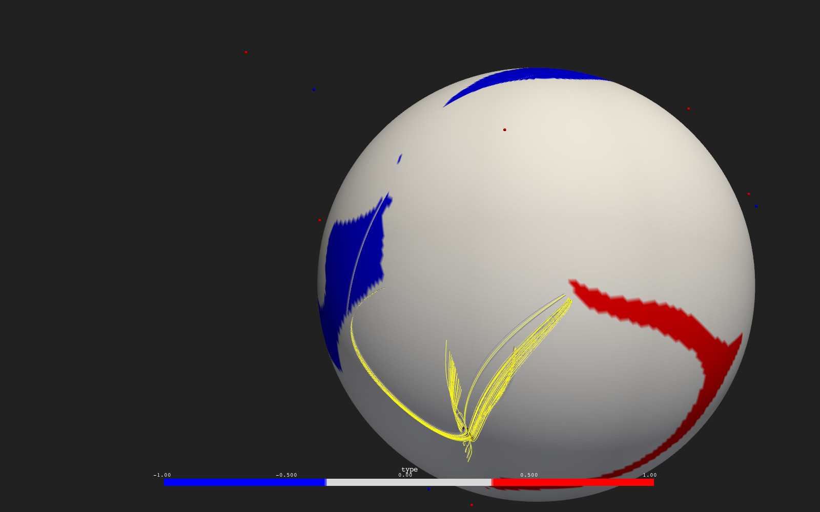
The output is a point cloud, a mesh dataset with one point per null and six arrays, in this order: type, spiral, det, residual, spine and fan_normal. A Plot colors by the first array, so with the psi_blue_gray_red colormap negative nulls are blue and positive ones red. The Plot uses style: points with render_points_as_spheres so that each null is visible as a sphere.

Picking one null

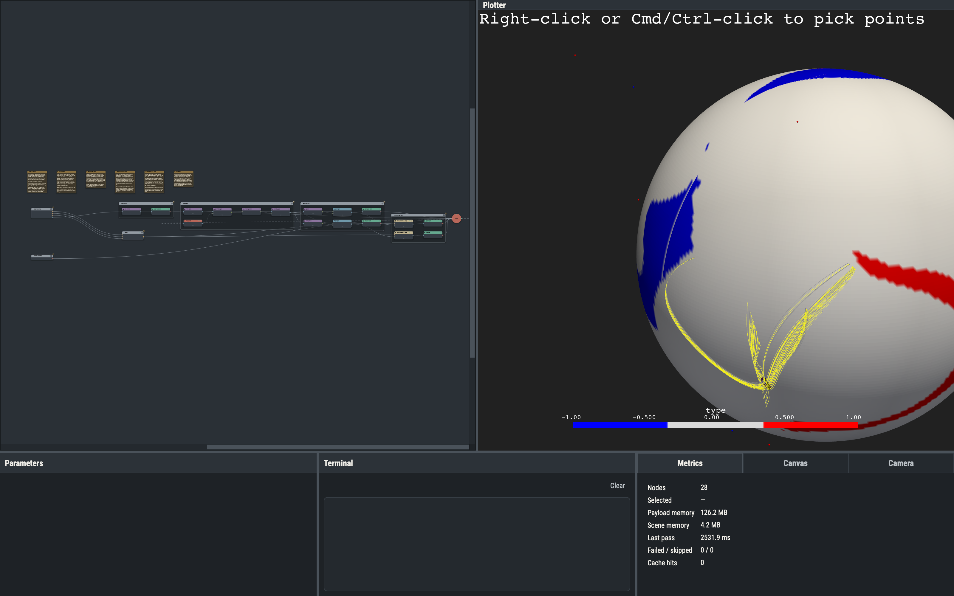
Pick Point returns the clicked position as a point. With Picker cell and Pick on set to the Null Points Plot, a click on a drawn null fires the holder. Nearest Index (Functions ▸ Structural) then finds which point of a stack is closest to a position: its x input takes the nulls (converted from a mesh back to a stack by From Mesh) and its position input takes the pick. Create Window repeats the single index into a window (i, i), and Stack Slice with Method index uses the window to return only that null, still carrying all six arrays. The solved session ships a pick on a null at about 1.3 R_sun, the lowest of the 26, and a saved view of the viewport that looks at it.

Spine and fan discs

Extract (Functions ▸ Structural) returns one component of a dataset as an array: spine and fan_normal of the selected null. A Disc (Datasets ▸ Shapes) is a ring of points around a center perpendicular to a normal; here the center is the selected null and the normal is the spine for one disc (Spine Disc) and the fan normal for the other (Fan Disc), with an inner radius of 0.005 and an outer radius of 0.03 R_sun. The discs are small so that every launch point lies close to the null, where the linear description above holds. For a null whose spine and fan normal nearly coincide the two discs nearly coincide as well; the more the null is skewed, the more they differ.

The disc points are launch points for Trace Domain, wired to the lps port exactly as in example 2.2. Lines from the Spine Disc are colored by polarity, and lines from the Fan Disc are drawn solid yellow, so the two sets stay distinguishable where they overlap.

Variations

• Picking a null with a higher r shows how the discs and lines change with the field strength around the null.
• Tracing along the spine of every null at once: Clip Scalar on type (value 0) keeps the positive or negative nulls, Warp By Vector displaces each null by ±0.05 along its spine, and the displaced points go to a Trace Domain lps.
• Volume Patch builds a small grid of the field around a null for a closer look at its structure.

Example 4.2 follows plasma along field lines.