Example 4.2: Flow Along Lines

Shortcuts are written Ctrl+…; macOS shows ⌘.

Goal

Resample traced field lines at equal steps of plasma travel time, so that a window of samples advances along each line with the flow, and drive that window with an animation.

Two fields, one set of lines

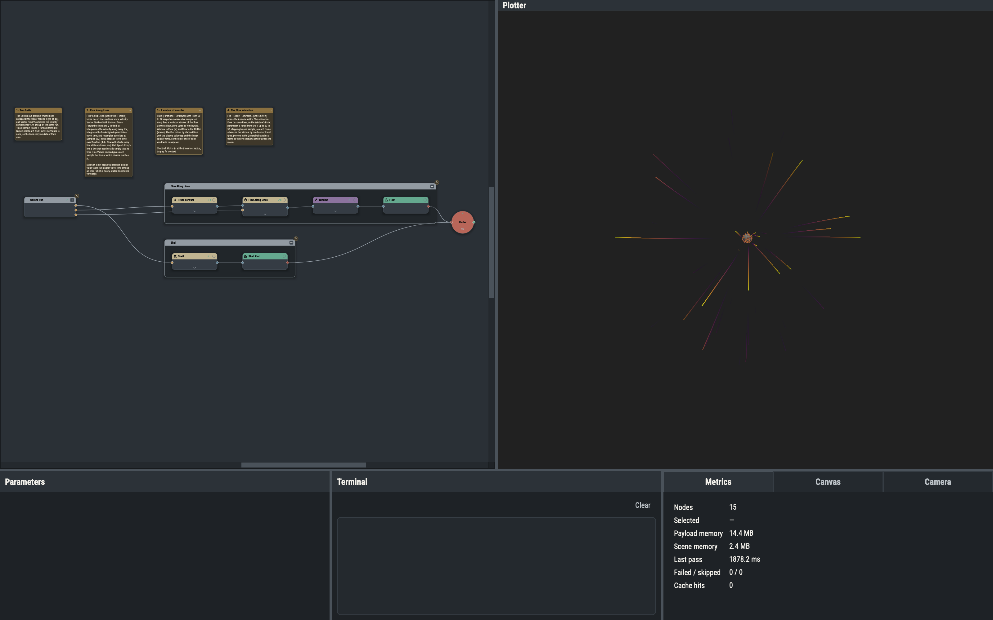
The magnetic field decides where a field line runs; the velocity decides how fast plasma moves along it. The scene therefore holds two vector fields from the same corona run: the Tracer is fed br, bt and bp, and a Vector Field named V combines vr, vt and vp (as in example 3.4, plain edges from the file nodes to the r, t and p ports of Vector Field). Trace Domain, with Direction forward, n 300 and r 1.05 R_sun, produces the lines. Its Line Values is none, since Flow Along Lines supplies its own values.

Flow Along Lines

Flow Along Lines (Generators ▸ Tracer) takes the traced lines on lines and a velocity field on field. For every line it interpolates the velocity at the line’s points, takes the component along the line, and integrates the reciprocal of that speed along the arc into a travel time. Each line is then resampled at samples equal steps of travel time up to duration, so sample k of every line is the position the plasma reaches after the same elapsed time.

• samples (97 here) is the number of points per output line; with a duration of 4 days it gives one sample per hour.
• duration must be set. A blank value takes the longest travel time among all lines, and a nearly stalled line makes that very large.
• flow chooses the direction. With flow starts every line at its upstream end, whichever way B was traced along it, so the window moves outward from the surface; Against flow starts at the downstream end and runs the other way, and each point is where the plasma was that many samples ago. The upstream end is the one the length-weighted mean speed along the line points away from.
• stall (Stall Speed) is the speed below which a segment stalls the particle: the line is NaN from that point on. 0 km/s lets every segment through.
• values (Line Values) sets what each sample carries: input passes the value arrays of the input lines through, elapsed gives the travel time to that sample (positive in both flow directions), and speed gives the field-aligned speed.

Travel time versus point index

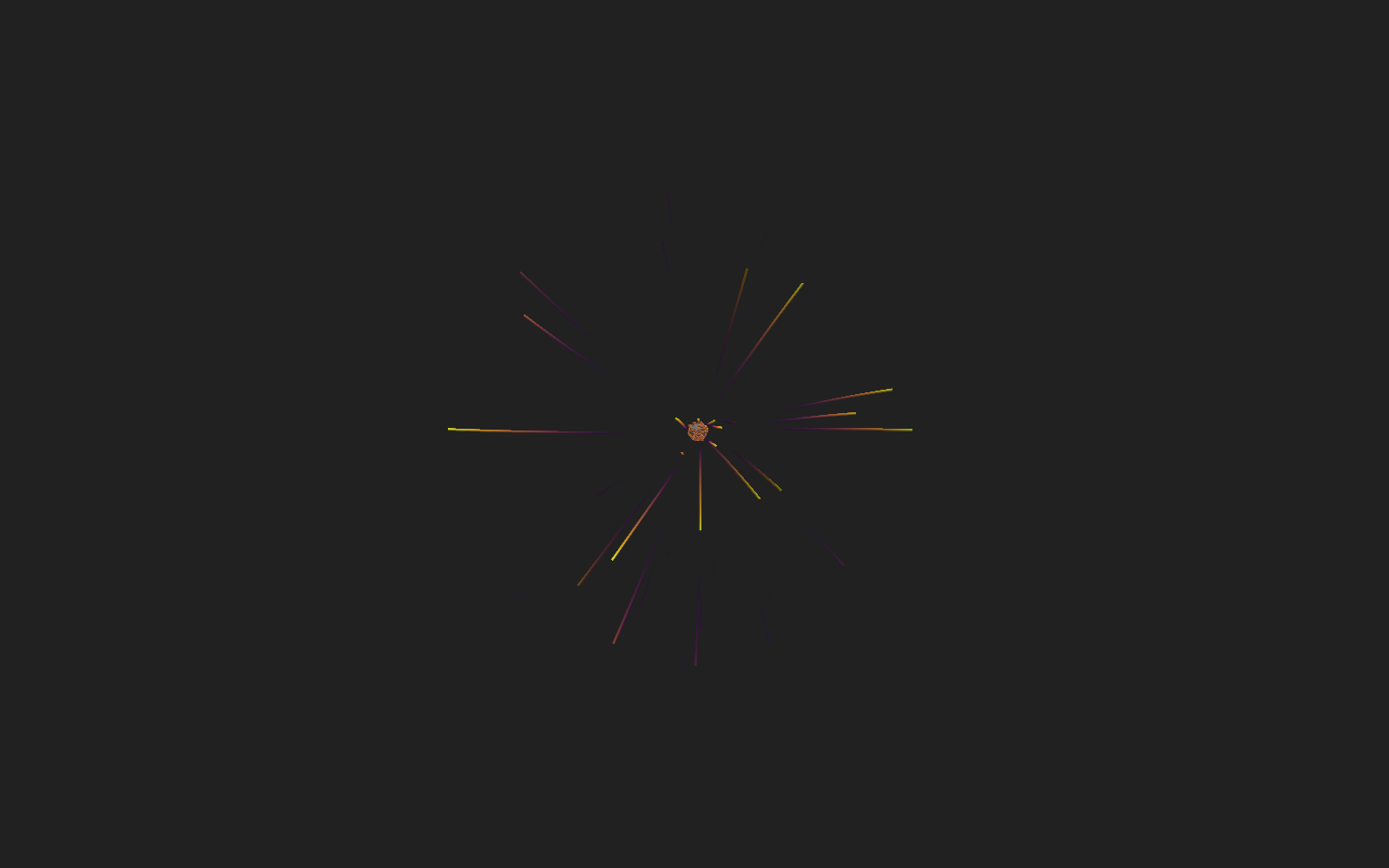
The input lines have unevenly spaced points, dense where the field is strong and sparse elsewhere, so the n-th point of a line says nothing about when the plasma gets there. After Flow Along Lines the n-th point of every line is the same elapsed time, so a Slice of consecutive indices (Functions ▸ Structural, Point 20 to 29 here, a ten-hour window) is a snapshot of where the plasma in each line is during those hours. The Plot colors by elapsed with the plasma colormap and opacity: linear, a ramp that makes the earlier end of each window transparent, and uses axis: 1, as for all line stacks, to join each line’s samples into a curve.

The Flow animation

The solved session carries one saved animation, Flow, with a single driver on the Window’s point parameter: a range from (0, 9) to (87, 96) with a stride of one sample. A window driver moves the pair lo–hi together, so every frame shows the next ten hours of flow. File ▸ Export ▸ Animate… (Ctrl+Shift+A) opens the Animate editor; Preview on the General tab applies one frame to the live session, and Render writes the movie. Example 4.4 describes the editor in full.

Variations

• Setting Line Values to speed colors each sample by the field-aligned speed instead of the time.
• Setting Flow to Against flow runs the window the other way along the lines.
• The Velocity Along Lines template in the library (File ▸ Browse Templates…) samples V on the lines with a Read method: points instead, which gives the velocity at the original points of each line without resampling it.

Example 4.3 exports a modified field and traces it again.