Plotting Points and Splines

This example demonstrates add_point(), add_points(), add_spline(), and add_splines() — the methods for rendering individual points, point clouds, single polyline paths, and bundles of splines from spherical coordinate arrays.

import numpy as np
from pyvisual import Plot3d

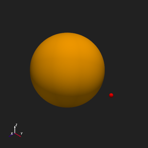
Single Point

add_point() renders a single location given as \((r, \theta, \phi)\) scalars. Here we place a marker at \(r = 1.5\,R_\odot\) on the equatorial plane (\(\theta = \pi/2\)) at 90° longitude (\(\phi = \pi/2\)).

plotter = Plot3d()
plotter.add_sun()
plotter.show_axes()
plotter.add_point(1.5, np.pi / 2, np.pi / 2, color='red', point_size=15)
plotter.show()

Static Scene

Interactive Scene

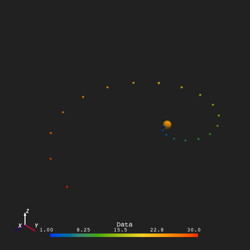
Point Cloud

add_points() accepts arrays of identical shape and renders them as an unconnected point cloud. Below, 20 points are placed along the equatorial plane (\(\theta = \pi/2\)), spiraling outward from \(r = 1\,R_\odot\) to \(r = 30\,R_\odot\) across a full longitude sweep. The data argument (here the radial distance \(r\)) controls the color mapping.

r = np.linspace(1, 30, 20)
t = np.repeat(np.pi / 2, 20)
p = np.linspace(0, 2 * np.pi, 20)

plotter = Plot3d()
plotter.show_axes()
plotter.add_sun()
plotter.add_points(r, t, p, r, point_size=5)
plotter.show()

Static Scene

Interactive Scene

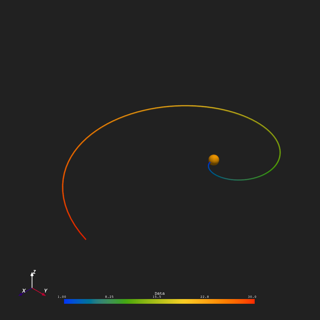
Single Spline

add_spline() draws a single line through a sequence of \((r, \theta, \phi)\) points. The example below traces an equatorial Archimedean spiral: the longitude \(\phi\) increases uniformly as the radial distance \(r\) grows from \(1\,R_\odot\) to \(30\,R_\odot\), approximating a Parker spiral in the ecliptic plane. The spline is colored by \(r\).

r = np.linspace(1, 30, 100)
t = np.repeat(np.pi / 2, 100)
p = np.linspace(0, 2 * np.pi, 100)

plotter = Plot3d()
plotter.show_axes()
plotter.add_sun()
plotter.add_spline(r, t, p, r, line_width=5)
plotter.show()

Static Scene

Interactive Scene

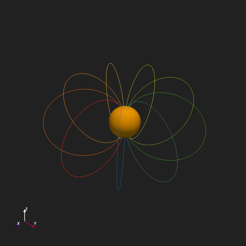
Bundle of Splines

add_splines() renders multiple splines from N-D coordinate arrays. Here, 10 meridional arcs connect the north and south poles at evenly spaced longitudes, tracing the surface of a sphere of radius \(5\sin\theta\,R_\odot\). The coordinate arrays have shape (10, 100); axis=1 declares that axis 1 (length 100) traces each individual spline path and axis 0 (length 10) enumerates the distinct meridians. Each spline is colored by its index.

n_lines, n_pts = 10, 100
r = np.tile(5 * np.sin(np.linspace(0, np.pi, n_pts)), (n_lines, 1))
t = np.tile(np.linspace(0, np.pi, n_pts), (n_lines, 1))
p = np.tile(np.linspace(0, 2 * np.pi, n_lines)[:, None], (1, n_pts))
data = np.arange(n_lines)

plotter = Plot3d()
plotter.show_axes()
plotter.add_sun()
plotter.add_splines(r, t, p, data, axis=1, show_scalar_bar=False)
plotter.show()

Static Scene

Interactive Scene