Arithmetic and NumPy Ufunc Support

SphericalMesh (and CartesianMesh) inherit a full arithmetic suite from _BaseFrameMesh. Standard Python operators (+, -, *, /, **, etc.) and NumPy ufuncs such as numpy.log10 and numpy.sqrt operate element-wise on the active scalar field and return a new mesh of the same type with the result as the active scalar. The coordinate arrays are never modified — only the data changes.

import numpy as np
from pyvisual import Plot3d
from pyvisual.core.mesh3d import SphericalMesh
from pyvisual.utils.data import fetch_datasets

br_file = fetch_datasets("cor", "br").cor_br

Build a Mesh

We initialize a SphericalMesh from the HDF file path, which triggers the file-path dispatch path (see Constructing a SphericalMesh for details on the three construction paths.

mesh = SphericalMesh(br_file)
mesh

Header	Data Arrays
SphericalMesh Information N Cells 10672572 N Points 10826790 X Bounds 9.997e-01, 3.042e+01 Y Bounds 0.000e+00, 3.142e+00 Z Bounds 0.000e+00, 6.283e+00 Dimensions 255, 142, 299 N Arrays 2	Name Field Type N Comp Min Max Data Points float32 1 -4.734e+01 4.797e+01 _PYVISTA_USER_DICT Fields 1 nan nan

Radial Flux Scaling

Multiplying by \(r^2\) removes the geometric falloff and converts \(B_r\) to the signed radial flux \(B_r r^2\). The coordinate arrays are unchanged; only the active scalar is updated.

mesh_r2 = mesh * mesh.r[:, None, None] ** 2
print(f"Br     range: [{mesh.data.min():.4f}, {mesh.data.max():.4f}]")
print(f"Br r^2 range: [{mesh_r2.data.min():.4f}, {mesh_r2.data.max():.4f}]")

plotter = Plot3d()
plotter.show_axes()
plotter.add_mesh(mesh_r2, cmap='seismic', clim=(-1, 1), opacity=0.5, show_scalar_bar=False)
plotter.show()

Static Scene

Interactive Scene

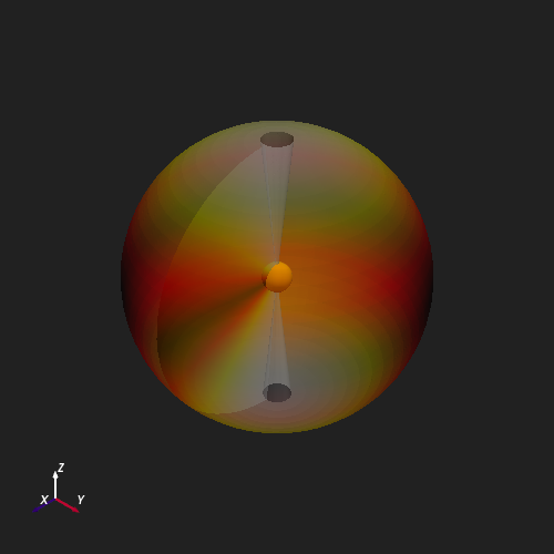
Br     range: [-47.3395, 47.9679]
Br r^2 range: [-47.3118, 47.9399]

NumPy Ufunc: np.log10

The __array_ufunc__() hook lets any single-output NumPy ufunc act directly on the mesh. numpy.log10 applied to \(B_r r^2\) converts the field to a logarithmic scale.

To account for the sign of \(B_r r^2\), we take the absolute value before applying the logarithm using the python built-in abs() function, which also supports the mesh type.

mesh_log = np.log10(abs(mesh_r2))
print(f"log10(|Br r^2|) range: [{mesh_log.data.min():.3f}, {mesh_log.data.max():.3f}]")

plotter = Plot3d()
plotter.show_axes()
plotter.add_mesh(mesh_log, cmap='rainbow', clim=(-1, 1), opacity=0.5, show_scalar_bar=False)
plotter.show()

Static Scene

Interactive Scene

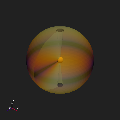
log10(|Br r^2|) range: [-6.870, 1.681]