Shells and Discs

This example demonstrates add_shell() and add_disc() — convenience methods for adding spherical shells and planar discs to the scene as reference geometry.

from math import pi
from pyvisual import Plot3d

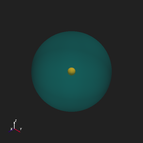
Source-Surface Shell

add_shell() adds a spherical shell defined by inner and outer radii, centered at an arbitrary spherical position. Here, a translucent shell at \(r = 10\,R_\odot\) represents the source surface — the heliospheric boundary beyond which coronal field lines are considered open.

plotter = Plot3d(off_screen=True, window_size=(500, 500))
plotter.show_axes()
plotter.add_sun()
plotter.add_shell(outer_radius=10, opacity=0.2, color='cyan')
plotter.show()

Static Scene

Interactive Scene

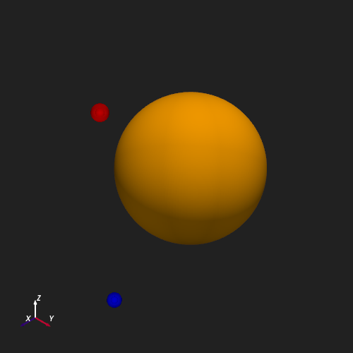
Positional Markers

Shells can also be placed at off-center positions to mark specific locations in the corona. The two small shells below are placed at symmetric latitudes in the northern and southern hemispheres at \(r = 2\,R_\odot\).

plotter = Plot3d(off_screen=True, window_size=(500, 500))
plotter.show_axes()
plotter.add_sun()
plotter.add_shell(2, pi / 4, 0, inner_radius=0.05, outer_radius=0.1,
                  color='red', opacity=0.8)
plotter.add_shell(2, 3 * pi / 4, 0, inner_radius=0.05, outer_radius=0.1,
                  color='blue', opacity=0.8)
plotter.show()

Static Scene

Interactive Scene

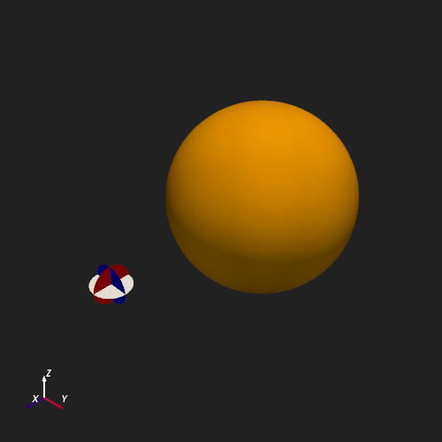
Local Basis Discs

add_disc() creates a planar disc whose normal is specified in the local spherical basis \((\hat{r}, \hat{\theta}, \hat{\phi})\) at the disc center. The three discs below illustrate each basis direction at \((r=2\,R_\odot,\,\theta=\pi/2,\,\phi=0)\): radial \(\hat{r}\) (blue), colatitudinal \(\hat{\theta}\) (white), and longitudinal \(\hat{\phi}\) (red).

disc_kwargs = dict(r=2, t=pi / 2, p=0, outer_radius=0.2)

plotter = Plot3d(off_screen=True, window_size=(500, 500))
plotter.show_axes()
plotter.add_sun()
plotter.add_disc(**disc_kwargs, normal=(1, 0, 0), color='blue')
plotter.add_disc(**disc_kwargs, normal=(0, 1, 0), color='white')
plotter.add_disc(**disc_kwargs, normal=(0, 0, 1), color='red')
plotter.show()

Static Scene

Interactive Scene