 PVA
Guide / Chapter 4
Nodes
A node is PVA’s atomic element: one operation with typed input ports, parameters and output ports. Every graph is built from them, and everything else in PVA, groups, templates and sessions, is a way of arranging and saving nodes. Editing a parameter or an edge recomputes nothing at once. It marks the affected nodes out of date, and a background pass later recomputes exactly what is needed. The Canvas covers adding and connecting nodes.
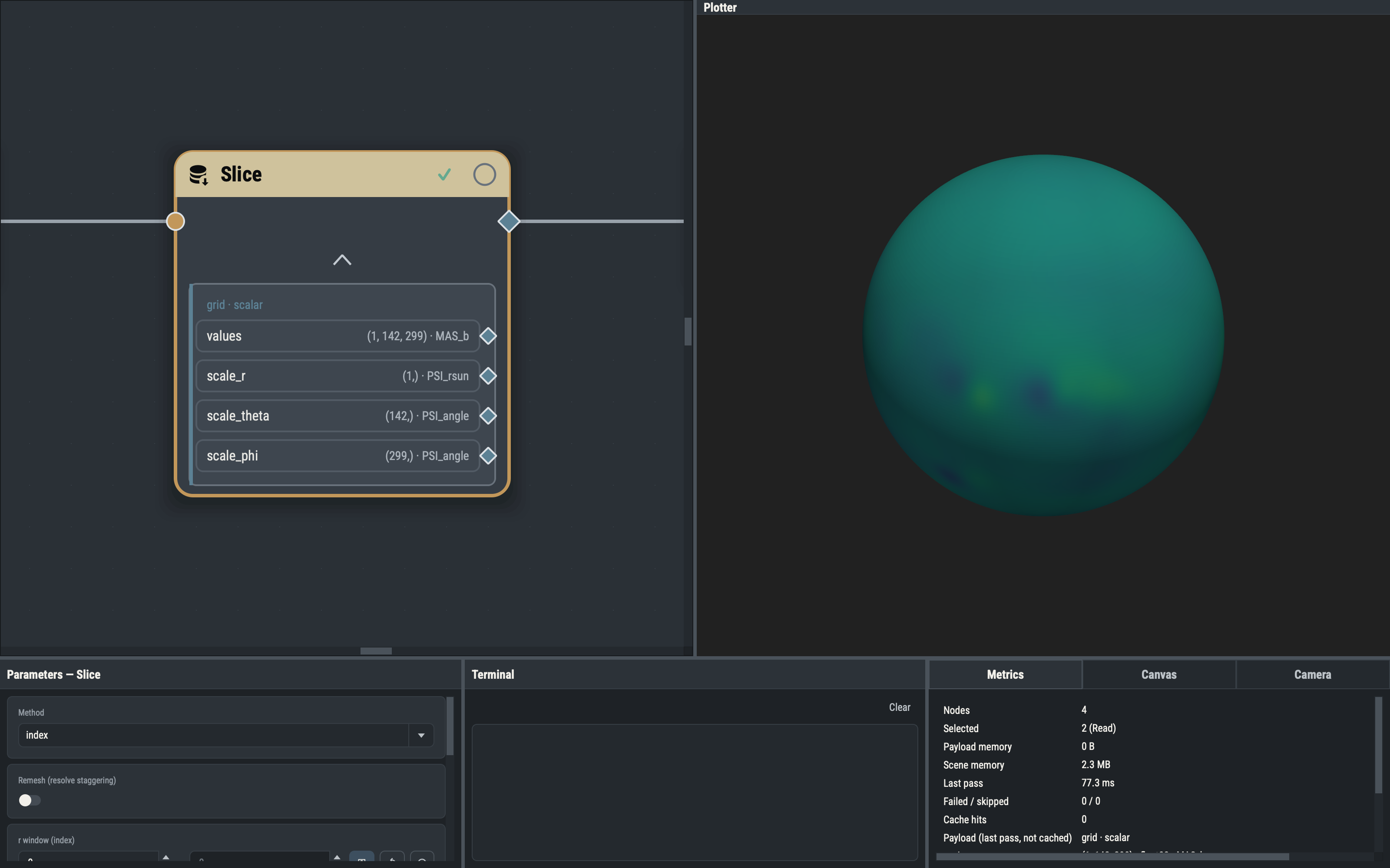
Anatomy of a node card
The card is a Slice node. Its title band is colored by node family (primitives, datasets, generators, materializers, functions, plot and export leaves, Plotters) and carries the type icon, the editable title, a state badge, a green dot while the node holds its result, and the cache override radio. Input ports are circles on the left (filled when required, outlined when optional), the output is a diamond on the right, and hovering a port names it. Below the ports a thin toggle strip, always reserved so a card never resizes when its first result arrives, expands the payload box; double-clicking the card toggles it too. A Plotter is a circle with a fixed frame caption (XYZ or RTP), and a collapsed group is a wide card showing only its boundary ports (Groups).
Ports
A port’s fill color gives its payload kind and its shape its role: required inputs are filled circles, optional inputs outlined circles, the output a diamond, and a component port a smaller diamond on a payload row. The kinds are primitives, datasets, generator handles, render payloads and events. A generator handle is a lazy engine handle (an opened file, for example) rather than data; a render payload (a Plot’s or Camera’s result) is a drawing instruction that only a Plotter accepts; a Plotter’s events output connects only to an event holder (Interactivity). One output can feed any number of inputs, but each input takes at most one edge, except ports that accept many, such as a Plotter’s scene.
Parameter ports
Most numeric parameters can be driven by an edge instead of a typed value. The drive port is an optional input that stays hidden until you add it with the parameter’s ⊕ button in the Parameters pane. While an edge feeds it, the connected value replaces the typed one at evaluation and the row’s caption reads linked (port while the port exists unconnected); disconnecting or removing the port restores the typed value. A one-element array, or a dataset whose value array has the right shape, is adapted automatically. Some nodes declare one port covering several parameters, such as a Tracer’s launch points or a Camera’s position. The row and caption vocabulary is in Parameter Pane.
Quiet optional ports
An optional input that drives no parameter is quiet: it is drawn on the card, and on a collapsed group’s boundary, only while it is relevant, connected or pinned. Examples are a Plot’s colors (relevant while color-by is rgba), Read’s lps (while the method is points), and the operand ports of the Filter and Replace nodes. Pin or unpin one from the Parameters pane’s Optional ports section; a pinned port is saved with the session.
The payload box
Once a node has evaluated, expanding its card shows a header line (a dataset’s caption, or a primitive’s shape, unit and dtype) and one row per addressable component with its (shape) · unit. Each row has its own diamond for connecting just that component. The box describes the last evaluation and dims while the node is not clean, since it no longer matches the inputs.
Reading values in a table
Click a component row (or a primitive’s header line) and then its table icon to open a read-only table window of the numbers. There is one window per node and component, cells are generated lazily so a million-point table is cheap, and a grid slab with more than two axes gets an index pin per extra axis. Selected cells copy as tab-separated text. The window shows the last evaluation and says so when the node has since changed. If the result is not in memory, opening the table turns the node’s cache override on and requests one evaluation; the override stays on until you click the radio.
Notes on a few families
The Nodes menu lists every type by family, and most are explained where they matter. Three families have rows worth knowing about before you meet them.
A reader (every file reader, such as MAS File, POT3D File, Map File or the Table readers) takes its data from one file, from a directory of files that match a pattern, or from the export cache folder; MAS File can also take a whole psi-data-utils sample run. A directory-style source reads one time step at a time, and Time Mode chooses the step. By Sequence uses a sequence number, By Date takes the file nearest a date, and By Time takes the file nearest an elapsed time in a unit you choose. The Directory and Cache Directory sources need the optional origin date t0 to give the sequence calendar dates for By Date; leave it blank otherwise. The Cache Directory source scans the folder that an Exporter’s Cache Directory destination writes to (see Files and Folders), and a reader watching that folder is marked out of date when an export writes a file there, so a reader picks up what an export in the same graph writes, with no reload.
The shapes under Datasets ▸ Shapes build geometry without a file. Grid Lines draws a spherical grid of lines from a range, a line count and a sample resolution for each of r, θ and φ. Equal endpoints collapse an axis, so narrow ranges make a box around one location, and a single radius makes a longitude-latitude graticule, a single meridian or a polar axis. Curtain spans a path, such as a spacecraft ephemeris, radially from an inner radius out to the path, which gives a ribbon surface to Sample through a field.
The Mesh Filters act on any dataset after converting it to a mesh. Besides clips, slices and contours, Rotate and Mirror turn a mesh about an axis or reflect it across a plane, carrying vector arrays along when Transform vectors is on, and Warp By Vector displaces every point by a vector array times a factor.
Status badges
The badge on the title band is the node’s state; groups use the same five.
| State | Meaning |
|---|---|
| Clean ✓ | The result is up to date with its inputs and parameters. |
| Dirty ! | An input, parameter or edge changed since the last evaluation; any result is out of date. |
| Pending … | A pass has been scheduled that will recompute this node; it has not started. |
| Evaluating ⟳ | The node is being computed right now. |
| Error ✗ | The last attempt failed; the message is in the Terminal. |
While a pass runs, Evaluating and Pending override the node’s own flags; otherwise Error outranks Dirty, which outranks Clean. A collapsed group shows the highest-ranking state among its members.
A node becomes dirty whenever something it depends on changes: a parameter, an edge connected or disconnected, an upstream node, or the removal of a node it reads. Dirtiness propagates downstream at once, so one edit marks the whole chain beneath it. Nothing recomputes during that walk; it only flips flags.
Evaluation is animated on the canvas: a computing card glows and a small dot travels along each incoming edge, the glow fades when the node finishes, and a failed node keeps a red border until retried or dirtied. The animation is styled by the [feedback] table of style.toml, which is read at startup.
Running the graph
What gets computed
Evaluation is demand-driven. A pass starts from root nodes whose results something needs and walks upstream, computing only out-of-date nodes and reusing clean results still in memory. The roots of an ordinary pass are every visible Plot connected to a Plotter’s scene port, every active Camera that has a source and is connected to a Plotter, and one-shot roots from explicit commands such as Evaluate and Export. A node that nothing visible depends on is not computed automatically; a hidden or unconnected Plot pulls nothing. To compute such a node anyway, select it and choose Evaluate.
Run, Evaluate and Auto
Three controls decide when a pass starts. Evaluate (CtrlReturn) evaluates the selected nodes and whatever upstream they need, as one pass. Run Graph (CtrlShiftReturn) ignores the selection and evaluates every ordinary root. The Auto Evaluate switch (CtrlE) is on at every launch and is not saved in sessions. While it is on, every implicit trigger requests a pass: a parameter edit, a new or removed edge, a pick or macro that changes a parameter, opening a session, undo and redo, and a render-only edit to a Plot. Changes in quick succession merge into one pass.
With Auto off, those triggers record the change and leave the graph visibly stale: the edited node and everything downstream turn dirty, and a Plot’s drawing stays as it was, marked pending. Turning Auto back on starts one catch-up pass. The switch never holds back explicit commands: Evaluate, Run Graph, an Exporter’s export, the Animate preview and the table window always run. An Exporter with Auto Export on is a root like a visible Plot: every pass that begins with it dirty (an upstream change, an edit to its own rows or a session load) writes its file again, and a pass with nothing changed writes nothing.
Background passes and cancellation
The GUI thread never evaluates. Every pass runs on one dedicated worker thread, so the canvas stays responsive and only one node computes at a time. At the start of a pass every out-of-date node it needs is marked pending; each becomes evaluating as it starts and clean or error when its result is applied. Each root’s result goes to the viewport as soon as it is ready, so a graph with several Plots fills in progressively.
A new edit during a pass supersedes it. The running pass stops at the next node boundary and a fresh one is queued; the node computing at that moment runs to completion and its result is discarded if the edit invalidated it. Dragging a spin box therefore never builds a backlog. Tracing is the exception: when the edit forces the tracer to rebuild, its subprocess is killed at once.
A node that fails gets the error badge and a red border, the message goes to the Terminal, and nodes that depend on it are not computed. A visible Plot that a superseded or failed pass did not commit stays pending, unless it is the node that failed, so the viewport never shows a half-updated result as current.
Slow-computation warning
When one node computes longer than a threshold, the Terminal logs one warning naming it (a trace node’s also gives the tracer timeout). The threshold is Settings ▸ Defaults ▸ Evaluation (3 seconds by default, 0 disables it), measured from when that node’s computation begins.
Dim stale meshes
The Render setting Dim stale meshes (off by default) lowers a pending Plot’s viewport opacity until it is recomputed. It is most useful with Auto off, where a drawing can stay stale for a long time. Volume renderings are never dimmed.
Caching
A node may keep its result in memory between passes, so later passes skip it and Deep Copy and the table window read it without recomputing. Editing anything the node depends on always discards the result.
The cache override radio on the card sets the policy. Auto (hollow ring) lets the application decide; Always keeps the result whatever the rule says; Pinned is fixed by the node type (Snapshot, Accumulator and the event holders) and cannot change. Click the radio on an unpinned node to switch between Auto and Always. The change never dirties the node and is one undo step. The green dot marks any node that currently holds its result.
The auto-cache rule
Under Auto, a node keeps its result after computing when more than one downstream node consumes its output (fan-out), or when this computation took longer than the Auto-cache threshold (Settings ▸ Defaults ▸ Cache, 0.1 seconds). Everything else is recomputed when needed. The rule is checked after each computation, so a node can start caching once it becomes expensive or gains a second consumer.
Display frames and units for vectors
A few parameters hold a position, such as a Camera’s position and focus or a Pick marker. They are stored in one fixed convention: spherical (r, θ, φ) with r in solar radii and both angles in radians. Macros, animation drivers, picks and connected ports all index those components. Two display policies control what you see and type; neither changes the stored value, any node’s result or the meaning of a saved file.
Display frame. A framed position row offers Cartesian (x, y, z), Spherical (r, θ, φ) and Longitude-Latitude (r, lat, lon), and each component has its own unit menu, so a point can show r in AU with angles in degrees. The session remembers frame and units per parameter. Switching frame changes only the view: no node becomes dirty and nothing recomputes. In Cartesian a point is meaningful only whole, so blanking one component blanks all three. Converting from Cartesian wraps φ into 0 to 2π, and the origin and polar axis map to zero angles. In Longitude-Latitude, lat is 90° minus θ and lon equals φ, with no wrapping or clamping.
Preferred units. Settings ▸ Defaults ▸ Units sets the length unit (R_sun, AU or km) and angle unit (deg or rad) that numeric fields, framed rows and the Camera pane display; values convert to and from the stored unit at the editor. A parameter with its own unit menu starts on the preferred unit when the node is created, and opening a session never converts a stored value.
See Parameter Pane for the layout of a framed vector and Camera Pane for the camera’s own frame controls.