 PVA
Guide / Chapter 15
Plot Node
The Plot node is how a dataset reaches the screen. It has one input, in, for the dataset and an optional colors port, and its output goes to a Plotter’s scene port (The Plotter). Most of what you see in a viewport, which form a stack takes, which array colors it, how translucent it is and how thick its lines are, is chosen by rows on this one node, so this chapter is the reference for those rows. The Plot reference page lists each row with its default and range.
From a Plot to an actor
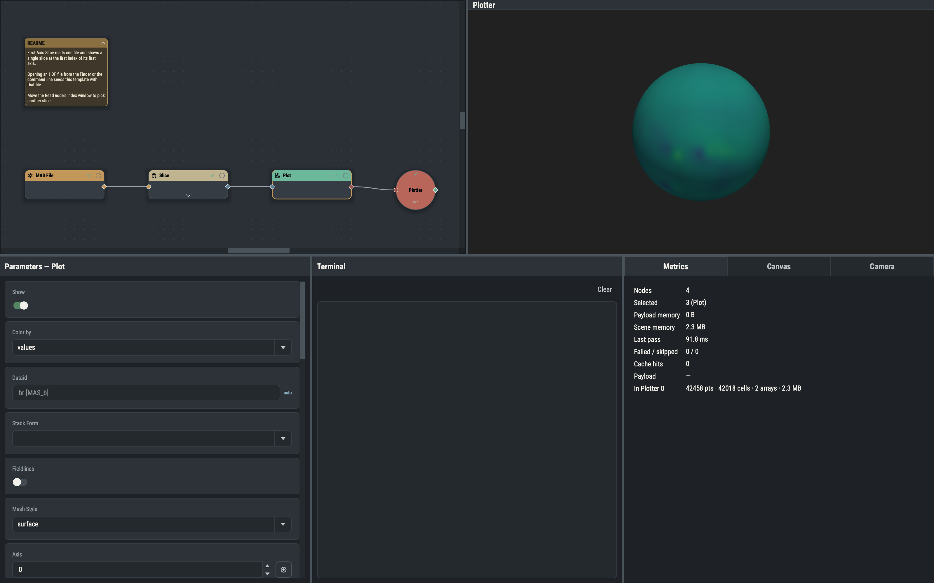
A Plot is scene-terminal: it does nothing until it is wired into a Plotter’s scene port, and it owns exactly one actor in each Plotter it is wired to. The Show switch is its demand-root flag: a visible Plot wired to a Plotter makes the graph evaluate everything upstream of it, and a hidden one pulls nothing (What gets computed).
Evaluating a Plot does not draw anything by itself. It produces the arguments that build a mesh and add it to a Plotter: the name of the drawing call, the input dataset exactly as it arrived (not converted), the declared arguments of that call (the array to color by, axis, Slice Type and Method) and the render rows. Rows left blank (Color limits, Solid color, Line width, Point size) are not sent, so the viewport’s defaults stand; every other row that applies is sent with its current value. The viewport then runs the call. The conversion from (r, θ, φ) to Cartesian positions and the conversion to 32-bit floats both happen inside that call, in the plotting library, which ends by adding a mesh to the Plotter. Plotter settings never re-evaluate anything, and editing a Plot row redraws its actor and never marks the graph out of date.
What the input decides
The dataset type picks the drawing call, and the call decides which rows apply.
| Input | Drawn as | Row that chooses the look |
|---|---|---|
| Grid with no free axis | One point. | None. |
| Grid with one free axis | A line. | None. |
| Grid with two free axes | A sheet. | None. |
| Grid with three free axes | A point cloud, splines or quad sheets. | Slice Type (points, splines, slices). |
| Stack | Points, splines, a reconstructed surface or the stack’s own faces. | Stack Form (points, splines, surface, mesh). |
| Surface dataset | Its own faces, by default. | Stack Form. |
| Mesh dataset | A surface, a wireframe or points. | Mesh Style (surface, wireframe, points). |
| Volume dataset | A volume rendering. | Blending and Shade. |
A free axis is a grid axis with more than one sample. A blank Stack Form defaults to splines for a traced field-line bundle or any other one-dimensional stack, so that a trajectory is a connected track; to mesh for a surface dataset; and to points otherwise.
Stack forms
A Plot draws a grid by its free-axis count and a stack by its Stack Form: points, splines (the default for traced field lines, with the Fieldlines option), surface (a sheet reconstructed through the points by the Method you choose) or mesh (a surface dataset’s own faces, with no reconstruction).
Warning. The
surfaceform triangulates every point of the stack on the main thread, and the cost grows roughly with the square of the point count on traced lines. The Plot refuses the form above 25,000 finite points with a Terminal error naming the count, so a Tracer’s output (a hundred lines of a few thousand points each) must be thinned first: put a Downsample node instridemode between the Tracer and the Plot, or trace fewer or shorter lines. Thesplinesandpointsforms have no such limit.
The mesh form draws a surface dataset’s own faces, so it fails with an error on any other stack. The Method row appears only for surface and chooses how the sheet is reconstructed through the points:
| Method | Reconstruction |
|---|---|
delaunay_2d | Projects the points onto a plane and triangulates them (the default). |
delaunay_3d | Builds a full volumetric tetrahedralization, then keeps its outer surface. |
reconstruct_surface | Reconstructs an implicit surface through the point cloud. |
With splines chosen, the Fieldlines switch draws the stack with the field-line renderer instead of the plain spline one. It starts on for a traced field-line payload, and it adds the Polarity coloring and Random coloring rows described under Coloring.
The axis parameter
Every builder that draws a stack or a three-dimensional grid first moves the dimension named by axis to the front of the coordinate arrays and then flattens the remaining dimensions. What that leading dimension means depends on the drawing.
Points, splines and field lines. axis is the dimension that runs along one line. Its length is the number of points per line, and the other dimensions enumerate the lines: a stack shaped (a, b, c) with axis 1 draws a × c lines of b points each. A traced bundle is shaped (lines, points per line), so it needs axis = 1. The default, 0, instead threads each line across the bundle, joining the first point of every trace, then the second, and so on; when a colors source has one row per trace and axis is 0, the error adds the hint that a field-line payload needs axis = 1. For the points form, axis changes only the order of the points, which matters for per-point colors.
Slices of a three-dimensional grid. With Slice Type slices, axis has the opposite meaning: it is the fixed dimension. Each index along axis becomes one quad sheet built from the other two dimensions, so a grid with n samples along axis draws n sheets. Grid axes are numbered r, θ, φ as 0, 1, 2:
axis | Fixed at each sheet | Sheet |
|---|---|---|
| 0 | r | A spherical shell, spanned by θ and φ. |
| 1 | θ | A cone, spanned by r and φ. |
| 2 | φ | A meridional half-plane, spanned by r and θ. |
A slab read as r × θ × φ and drawn as slices with axis 1 therefore gives one cone sheet per θ. Shared Controllers draws its slices with axis 0 and 2. With Slice Type points or splines, axis is the line dimension again: for splines it is the dimension each spline runs along, and the other two dimensions enumerate the splines.
Per-point rows and curves. Because axis fixes the order in which points are drawn, per-point color rows, whether from an rgba source or built for a solid color shaded by a function, are reordered to match it before they reach the viewport, and the point and cell counts that a custom opacity curve or an rgba source is checked against also follow axis.
For a worked example, the field-line Plot of Reconnection Between Steps sets axis: 1, because its stack is a traced bundle of lines.
Coloring
Color by chooses where color comes from. The row appears when the input has a value array or the colors port is connected.
- values colors by one value array. dataid names the array; a blank dataid uses the payload’s first value array, shown as its name with a unit, such as
rho [g / cm3]. With several arrays, such as a vector grid, dataid selects any of them by name (values_r,values_theta,values_phi); an unknown name falls back to the first. A stack with no value arrays but a time scale is colored by time. The colormap rows (Colormaps) apply, and the scalar bar. - solid draws one color, Solid color, and ships no value array to the viewport, so the color wins over any scalars. The colormap rows are hidden and not sent. A payload with no value array at all is always solid, and shows Solid color without a Color by row.
- rgba takes the colors from the
colorsport: anN × 3orN × 4array (floats from 0 to 1, oruint8), or a stack withr,g,band optionalavalue arrays, matched by name without regard to case (red,green,blueandalphaalso work). The Colormap, Random Colors and Compose RGBA nodes under Functions ▸ Colors build such rows.
The rows of an rgba source must match what the call draws: one row per point or one row per cell. The Plot compares the row count with the point and cell counts of the geometry it will build and colors points or cells accordingly; a count that matches neither fails with an error that gives both counts. When the colors carry an alpha channel the Opacity row is hidden, because the colors already hold it. The surface Stack Form cannot take rgba colors (use mesh, or convert with To Mesh first), and a named transfer function is refused as the opacity.
Field lines. With Fieldlines on, two switches pick a coloring preset. Polarity coloring (shown while coloring by values) colors each line by its open or closed polarity state with the polarity palette. It needs the payload’s first value array to be polarity, which a Tracer produces when its Line Values is set to polarity; the Plot fails with that advice otherwise. The preset owns the colormap rows, so they are hidden, but Show scalar bar stays available. Random coloring (shown while coloring solid, or when the payload has no values) gives every line its own random hue.
Colormaps
The colormap rows apply while coloring by values:
- Colormap maps the colored array to colors. It is a stock colormap, or
@namefor a custom colormap of your own (Custom colormaps). The default comes from Settings ▸ Defaults ▸ Render. - Reverse colormap reverses it, stock or custom.
- Color limits are the data range that maps onto the colormap. Blank uses the finite range of the colored array.
- Log scale maps values to colors on a logarithmic scale; values below zero take the lowest color.
- Show scalar bar draws the color bar. It stays available under Polarity coloring.
All of them are hidden, and not sent, while coloring solid or rgba. To color by an RGBA array you compute, build the rows with the Colormap node, which mirrors the Plot’s colormap, reverse, limits and log-scale rows and adds an optional per-row alpha, and wire the result into colors.
Custom colormaps
A Plot’s Colormap, and the Colormap node’s, can name a custom colormap as @<name>: a gradient of color stops over the colored scalar’s range. The Colormap row has an Edit… button beside the picker, which opens a modal editor listing saved colormaps beside a name, an interpolation and a gradient strip with its stops underneath. Your saved colormaps appear in the picker after the stock ones. Reverse works on them like any other colormap. The Settings window’s default colormap and the Plotter theme keep the stock catalog only.
-
Gestures. Drag a stop to move it along the range (the two end stops only change color). Double-click empty space to add a stop, colored from the gradient at that position. Double-click a stop to pick its color. Delete an inner stop by right-click, or select it and press Delete.
-
Interpolation.
linearblends in sRGB,stepholds the color of the stop to the left, andperceptualblends in Oklab so the midpoint of two colors keeps an even lightness. -
Based on. The Based on picker and Stops count start the gradient from any stock colormap sampled at that many stops (linear). The flip button mirrors the gradient left to right.
-
Stop row. The selected stop’s position, color swatch and
#rrggbbhex field edit it directly. A narrow grayscale band under the gradient shows its lightness, so you can see whether a map holds up in grayscale. -
Save stores the colormap under the name. A blank name prompts for one, and replacing a saved colormap you have edited asks for confirmation first.
-
Save As… asks for a new name and refuses a blank or taken one.
-
Delete removes the colormap from your library.
-
Use saves, closes and sets the row to
@<name>.
Colormaps live in colormaps.yaml in the user settings folder (Files and Folders). A name may not contain a colon. An unknown name fails with unknown colormap '@<name>': not in the library or this session.
Opacity
Opacity is one row that takes three kinds of value.
- A number from 0 to 1, applied evenly to the whole drawing. The default comes from Settings ▸ Defaults ▸ Render.
- A transfer function name, which makes opacity depend on the colored value. The function is spread over the colormap’s range, the Color limits when set and otherwise the range of the colored array: the lowest value gets the function’s first opacity and the highest its last. The names are the ones pyvista provides:
| Name | Shape |
|---|---|
linear | A straight ramp from transparent at the lowest value to opaque at the highest. |
geom | A geometric ramp: nearly transparent over most of the range, rising steeply at the top. |
sigmoid | An S-curve, 1 / (1 + exp(-x)) for x from -10 to 10. |
sigmoid_1 to sigmoid_10, sigmoid_15, sigmoid_20 | The same S-curve over x from minus to plus the number in the name; a larger number gives a sharper step from transparent to opaque. |
foreground | Only the lowest value is transparent; everything above it is opaque. |
linear_r, geom_r, sigmoid_r, sigmoid_3_r to sigmoid_10_r | The reverse of the matching name: opaque at the lowest value. |
- A custom
@namecurve that you draw yourself (Custom opacity functions). It is sampled into a short list of opacities, 128 values (4 under Polarity coloring), lowered until the length differs from every point and cell count of the geometry, because pyvista reads an opacity array of exactly such a length as per-element opacity. The list is spread over the colormap in the same way as a named function.
A transfer function or curve needs a value array to map over. A three-dimensional grid drawn as slices, splines or points with a transfer function acts as a “faux” volume, showing dense values and fading the rest. A function cannot be combined with rgba coloring.
When coloring solid, a function fades the solid color by value instead of being constant: the node builds RGBA rows with the constant color and, for each point or cell, an alpha from the function at the colored array’s value over its Color limits, and sends those rows. dataid and Color limits apply then, NaN values are fully transparent, and the surface Stack Form is refused.
Custom opacity functions
A Plot’s opacity can name a custom opacity function as @<name>: a curve mapping the colored scalar’s range (left to right) to opacity (bottom to top). Edit opens a modal editor listing saved functions beside a name, an interpolation (linear, step or smooth) and the curve. Drag a point to move it (end points only vertically), double-click empty space to add one, and delete an inner point by right-click, or select it and press Delete. A Shape menu starts the curve from 13 analytic shapes at a chosen point count, and the two flip buttons beside it mirror the current curve left to right or invert it, so an inverse ramp, a notch or a left-handed step is one click from its counterpart.
- Save stores the curve under the name, replacing a function of that name.
- Save As… asks for a new name and refuses a blank or taken one.
- Delete removes the function from your library.
- Use saves, closes and sets the Plot’s opacity to
@<name>.
Functions live in opacity-functions.yaml in the user settings folder (Files and Folders). A function also applies to a solid color, which then fades by the data value (over the data field and color limits) instead of being constant. Color-by rgba refuses a function, and an unknown name fails with unknown opacity function '@<name>': not in the library or this session.
Lines, points, spheres and tubes
Which of these rows a drawing shows follows from its look. One rule decides it, the same one that decides what is sent (Which rows apply):
| Look | Drawn by | Rows |
|---|---|---|
| Point | A single point, the points form, Slice Type points, Mesh Style points | Point size, Render points as spheres |
| Line | A line, the splines form and field lines, Slice Type splines, Mesh Style wireframe, or a mesh made only of lines | Line width, Render lines as tubes |
| Surface | A sheet, the surface and mesh forms, Slice Type slices, Mesh Style surface | Show edges |
Turning on Show edges for a surface also shows the line rows, since the edges are lines.
- Line width and Point size set the thickness of lines and the size of points. Blank leaves the viewport’s default.
- Render points as spheres draws each point as a shaded, lit sphere instead of a flat square dot.
- Render lines as tubes draws each line as a shaded tube whose diameter is the line width, lit and depth-correct, instead of a flat screen-space line. Tubes are an explicit opt-in on this node, off by default.
Both are done by shaders as impostors: no sphere or tube geometry is added, so the mesh stays the size it was, but every covered pixel is shaded. A bundle of several hundred lines drawn as tubes, such as the one in the Reconnection template, can be noticeably slower than flat lines, so turn tubes on only for lines that need them.
Volumes
A volume dataset, such as the output of Volume Patch, is drawn by volume rendering instead of as a mesh. It is always colored by its one value array, so it has no Color by, Solid color or look rows. The rows that apply are Show, Opacity, dataid, the colormap rows and two volume-only rows. Blending chooses how the samples along each ray combine into one pixel:
| Blending | Result |
|---|---|
composite | Samples are blended front to back by their opacity (the default). |
maximum | Each pixel shows the largest sample along its ray. |
minimum | Each pixel shows the smallest sample along its ray. |
additive | The samples along the ray are added. |
average | The samples along the ray are averaged. |
Shade lets the volume mapper apply lighting. It is off by default, and some blendings, such as maximum, ignore it. A wired colors port is ignored for a volume, and a volume cannot be drawn in an RTP Plotter.
Which rows apply
The Plot form shows only the rows that matter for the current input and choices, and a row that is hidden is not sent. This is the one node family where the two are the same: on every other node a hidden row still forwards its value. For example, switching Color by to solid hides the colormap rows and stops sending them, and switching the Stack Form from points to splines swaps Point size for Line width. If nothing is connected to in, or the connected nodes offer more than one kind of dataset, the form shows every row.
The Plot reference page lists every row with its default, range and a one-line description.